Chapter 9: Classical signal processing filters
In Chapter 8 we have introduced, among other ideas, Butterworth filters of the 1st kind. In this chapter we are going to construct further similar filter types by allowing the amplitude response to have ripples of equal amplitude (a.k.a. equiripples) in the pass- or stop-band, or in both. These filters as well as Butterworth filters of the 1st kind are the filter types used in classical signal processing. They have somewhat less prominent role in music DSP, therefore we first concentrated on other filter types. Still, they are occasionally useful.
9.1 Riemann sphere
Before we begin discussing equiripple filters we need to go into some detail of complex algebra, concerning the Riemann sphere and some derived concepts. The key feature of the Riemann sphere is that infinity is treated like any other point, and this (among with some other possibilities arising out of using the Riemann sphere) will be quite helpful in our discussions. It seems there are a number of slightly different conventions regarding the Riemann sphere. We are going to introduce now one particular convention which will be most useful for our purposes.1
Given a complex plane we introduce the third dimension, thereby embedding the plane into the 3-dimensional space . The and axes coincide with and axes, the axis is directed upwards. The Riemann sphere will be the sphere of a unit radius (Fig. 9.1). Thus, the intersection of the Riemann sphere with the complex plane is at the “equator” which in terms of is simply the complex unit circle . The center of projection will be at the “north pole” of the Riemann sphere, which thereby is the image of . Respectively, the complex unit circle coincides with its own projection image on the Riemann sphere.
We will denote and refer to the points on the Riemann sphere by the complex values that they represent. E.g. the “north pole” will be simply denoted as , the “south pole” as , the point on the “zero meridian” as , the point on the meridian as etc. Some of these points are shown on Fig. 9.1.
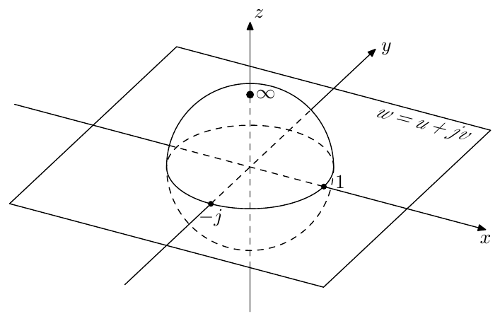
Figure 9.1: Riemann sphere.
Real Riemann circle
The 2-dimensional subspace of the space in Fig. 9.1 contains just the real axis of the complex plane and the real axis’s image on the Riemann sphere which is a circle of unit radius (Fig. 9.2). It will be intuitive to refer to this circle as the real Riemann circle.
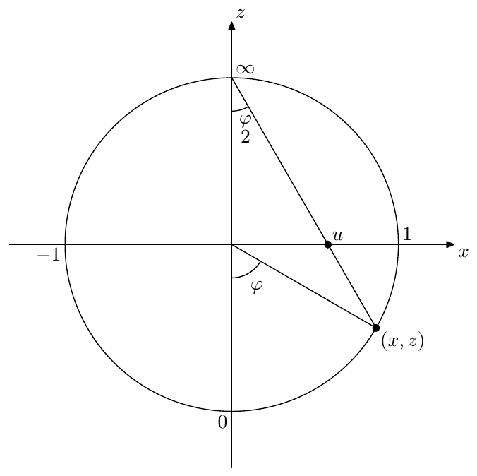
Figure 9.2: Real Riemann circle. The 0, 1, , -1 labels denote the points on the circle which correspond to these values.
We can use the polar angle (defined as shown in Fig. 9.2) as the coordinate on the Riemann circle. One of the reasons for this choice of definition of are the following convenient mappings between and :
Also, if we restrict to , then
From Fig. 9.2, using some basic geometry it’s not difficult to find that and are related as
and that
By introducing the “homogeneous” coordinate the equation (9.2a) can be rewritten in a more intuitive form:
Conversely, using Fig. 9.2 and equation (9.1) we have
Symmetries on the real Riemann circle
Certain symmetries between a pair of points on the real axis correspond to symmetries on the real Riemann circle. Specifically, from (9.1) we obtain:
or, by restricting and to
Fig. 9.3 illustrates.
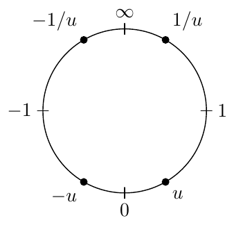
Figure 9.3: Symmetries of the values on the real Riemann circle.
Coordinate relationships for the Riemann sphere
The equations (9.2) and (9.3) generalize to the 3-dimensional space containing the complex plane and the Riemann sphere in an obvious way as:
and
The equation (9.1) can be generalized if we restrict to , in which case
In principle we could also introduce the spherical azimuth angle, which is simply equal to , but we won’t do it in this book.
Imaginary Riemann circle
The subspace of the space in Fig. 9.1 contains just the imaginary axis of the complex plane and the imaginary axis’s image on the Riemann sphere which is a circle of unit radius . We will refer to this circle as the imaginary Riemann circle.
There are no essential differences to the real Riemann circle. The same illustrations and formulas hold, except that we should use in place of . Fig. 9.4 provides a simple illustration of the circla and its symmetries. Note that the reciprocal symmetries change sign if expressed in terms of the complex variable , since .
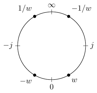
Figure 9.4: Symmetries of the values on the imaginary Riemann circle, where , .
9.2 Arctangent scale
From the Riemann circle one can derive a special scale which will be useful for plotting function graphs with interesting behavior around infinity. One commonly known special scale is a logarithmic scale which maps the logical values to the geometric positions on the plot. In a similar fashion, we introduce the arctangent scale
which is using the polar angle of the real Riemann circle as the geometric position . It is easy to notice that (9.9) is equivalent to (9.1), where we have in place of and in place of .
The actangent scale warps the entire real axis into the range . Due to the periodic nature of the Riemann circle’s polar angle it is not unreasonable to require the scale to be periodic as well, in which case we can also support the value which will map to .
Treating the infinity like any other point, the arctangent scale provides a convenient means for plotting the functions where the range of the values of interest includes infinity. E.g. we could plot the graph of the cosecant function using the arctangent scale for the function’s value axis, as illustrated by Fig. 9.5
Symmetries in the arctangent scale
The symmetries of a graph plotted in the arctangent scale are occurring in agreement with Riemann circle symmetries (9.4) and (9.5) (illustrated in Fig. 9.3). Specifically:
- Mutually opposite values are symmetric with respect to points and .
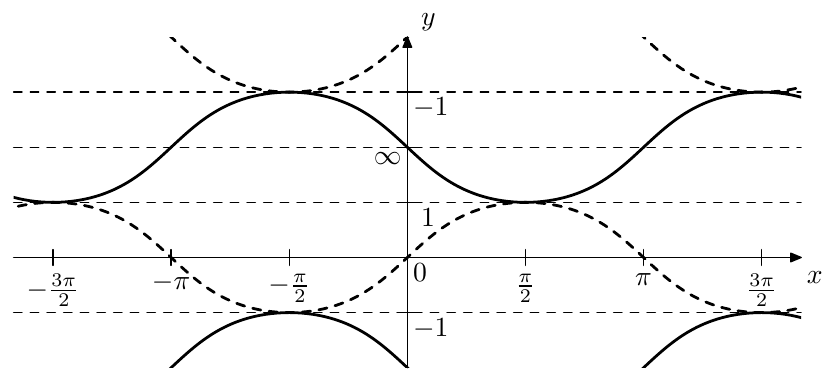
Figure 9.5: Graphs of (dashed) and (solid) using arctangent scale for the ordinate.
-
Mutually reciprocal values are symmetric with respect to points and .
-
Values whose product is map are spaced by the distance equal to the half of the arctangent scale’s period, that is e.g. to the distance between and or between and .
One can observe all of these properties if Fig. 9.5, where the third property can be observed between the and the half-period-shifted .
9.3 Rotations of Riemann sphere
We are going to introduce two special transformations of the complex plane:
where . It is easy to check by direct substitution that , that is the transformations and are each other’s inverses.2 As we shall see, are simply rotations of the Riemann sphere by in two opposite directions.
Letting where and are the real and imaginary parts of , we have
That is
On the other hand,
and
from where by (9.7d)
Then, using (9.7) we obtain
That is , , which is simply a rotation by around the axis in the direction from the (positive) axis towards the (positive) axis. Thus simply rotates the Riemann sphere around the imaginary axis of the complex plane by in the direction from to , or, which is the same, in the direction from to (where by , and we mean the points on the Riemann sphere which are the projection images of , and respectively). The points are thereby untouched, which can be also seen by directly evaluating . The transformation being the inverse of simply rotates in the opposite direction.
In terms of the real Riemann circle clearly correspond to a counterclockwise (for ) or clockwise (for ) rotation by (Fig. 9.6).3 Respectively, in the arctangent scale they correspond to shifts by a quarter of the arctangent scale’s period.
The imaginary Riemann circle is rotated into the unit circle , which is its own image on the Riemann sphere. Therefore for the polar angle from Fig. 9.2 becomes the polar angle in the complex plane (since and since ), therefore and by (9.1) we have
This can also be verified by direct substitution, where it’s easier to use the inverse transformation:
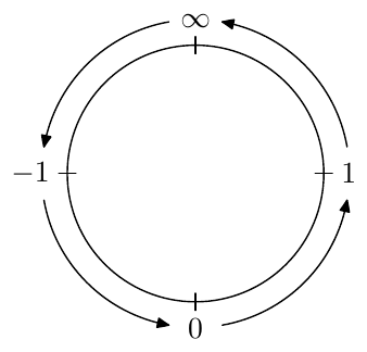
Figure 9.6: Transformation of the real Riemann circle by .
For the polar angle gets mapped into . Conversely a polar angle equal to will be mapped into , thus
Summing up:
Note that (9.12) do not simply give the inverse versions of (9.11), but also reflect the fact the complex unit circle gets rotated into the imaginary Riemann circle.
Symmetries
The transformations of symmetries by can be derived in an intuitive way from the symmetries on the real Riemann circle and the arctangent scale and from the fact that these transformations are rotations of the real Riemann circle or (equivalently) shifts of the arctangent scale by the scale’s quarter period, if we assume .
Particularly, a rotation of the real Riemann circle maps and to and vice versa. Respectively, points on the Riemann circle which are symmetric relatively to and map to points symmetric relatively to and vice versa. Thus, mutually opposite values map to mutually reciprocal values and vice versa:
Fig. 9.7 illustrates, where more properties are immediately visible. E.g. one could notice that are obtained by rotating by , therefore the results are apart, which means:
or that rotating the opposite points by in opposite directions produces opposite points:
etc.
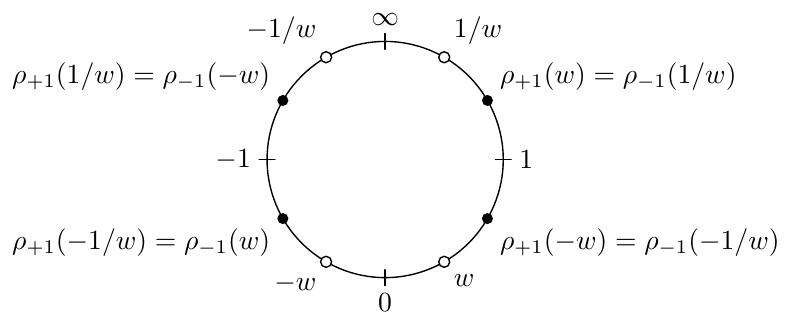
Figure 9.7: Symmetries of the transformations on the real Riemann circle, where they represent rotations.
The formulas (9.13), (9.14) and other similarly obtained symmetry-related properties of work not only for but actually for any which can be verified algebraically. However, the interpretation of these symmetries in terms of the real Riemann circle obviously works only for .
The imaginary Riemann circle gets rotated by into the complex unit circle, where the results of the two transformations are thereby symmetric relatively to the imaginary axis. Fig. 9.8 illustrates some of the symmetries arising out of this rotation. More illustrations of this kind can be created, particularly for the transformation of the values lying on the complex unit circle, but the ones we are already having should be sufficient for our purposes in this book.
Unit circle rotations
The Riemann sphere rotations can be described as rotations of the Riemann sphere around the imaginary axis or as rotations of the real Riemann circle. Similarly the Riemann sphere rotations around the vertical axis can be thought of as rotations of the unit circle.
Apparently, such rotations are simply achived by a multiplications of complex values by a unit-magnitude complex constant, where we are not restricted to rotations by multiples of . We won’t need a special notation for this transformation and will simply write
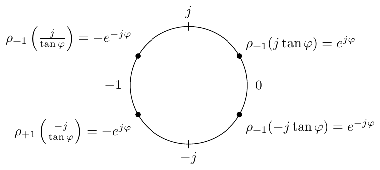
Figure 9.8: Symmetries of the results of the transformation of the imaginary axis (lying on the complex unit circle).
Obviously
The rotations by and are simply multiplications by and respectively.
There is not much more to say in this respect as this rotation is pretty trivial.
Imaginary rotations
We could also wish to rotate the imaginary Riemann circle. We will denote the respective transformations as , where the subscript, as with , denotes the image of the zero after the transformation.
We could rotate the imaginary circle by doing the three steps in succession:
-
First, we rotate the Riemann sphere by around its “vertical” axis, thereby turning the imaginary Riemann circle into the real Riemann circle, where is transformed into respectively, while and stay in place. Such rotation is simply achieved by multiplying by .
-
Now we apply to rotate the real circle.
-
We convert the real circle back to the imaginary one by multiplying the rotation result by .
Therefore we simply have
(where the second expression is obtained in the same way as the first one, except that we rotate the Riemann sphere in the other direction, both vertically and horizontally).
In order to distinguish between and we could refer to the former as real rotations of the Riemann sphere and to the latter as imaginary rotations of the Riemann sphere.
9.4 Butterworth filter revisited
In Chapter 8 we have developed the lowpass Butterworth filters of the 1st kind (also simply known as Butterworth filters) as a Butterworth transformation of the 1-pole lowpass filter, where we also mentioned that the tranditional definition of the Butterworth filter simply defines the (lowpass) Butterworth filter as a (stable) filter whose amplitude response is
Apparently both definitions are equivalent.
We could generalize this idea by replacing in (9.17) by some other polynomial function :
The practical application of (9.18) essentially follows the steps of the Butterworth transformation of the 1st kind, which includes solving to obtain the poles of and then discarding the right-semiplane poles, thereby effectievely obtaining the desired transfer function expressed in the cascade form. Note that there are two implicit conditions which need to be fulfilled in order for this procedure to work:
-
There is the symmetry of the poles of with respect to the real axis: if is a pole then so is (where may be the same pole as if is real). This is necessary in order for to be a real function of .
-
There is the pairwise symmetry of the poles with respect to the imaginary axis: if is a pole then is another pole (it must be another pole even if , in which case it simply means that the pole is duplicated). This guarantees that we can split the poles into the left- and right-semiplane halves with identical contributions to the amplitude response. Therefore by discarding the right-semiplane half of the poles, we effectively go from to .
We could expect that these properties will not be fulfilled for an arbitrary . However, let’s require that
-
The function is a real function of .
-
The function is odd or even.
The readers can convince themselves that under these restrictions the poles of defined by (9.18) will have the necessary symmetries with respect to the real and imaginary axes.
Rational
We could allow to be not just a polynomial but a rational function. In this case has not only poles, but also zeros at locations where has poles and respectively the denominator of turns to , which means that both and turn to zero. In order to see that the multiplicities of the zeros of are equal to the multiplicities of the respective poles of of simply consider
Thus the set of zeros of is the duplicated set of zeros of , however after switching to we should drop the duplicates, being left only with a single set of zeros of , which are the poles of . Note that shouldn’t have more zeros than poles, which means that the order of the denominator of should not exceed the order of the numerator of .
In order for to be real, its zeros must be conjugate symmetric, which will be ensured if is real odd or even function. Indeed, in this case the poles of are both conjugate symmetric and symmetric with respect to the origin, which implies that they are also symmetric with respect to the imaginary axis, which is the same as the symmetry with respect to the real axis.
Representations of linear scaling
We are now going to develop another way of looking at the Butterworth filter generating function . It will be highly useful with other functions occurring in place of in (9.18).
Let . Since , we can write
Introducing auxiliary variables and we can rewrite (9.19) as a set of equations:
which also allows to define implicitly as a function satisfying the equation
We could consider and as representations of and , where the connection between the preimages and and their respective representations and is achieved via the exponential mapping (Fig. 9.9). In terms of preimage domain the function is simply a multiplication by .
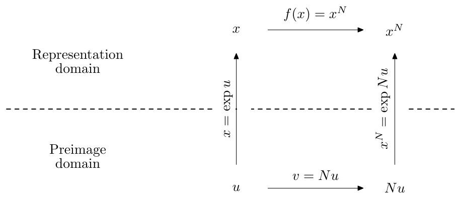
Figure 9.9: The preimage and representations domains.
Now consider that the function is periodic in the imaginary direction:
Therefore preimages are -periodic, that is if is a representation of , then so is (Fig. 9.10).
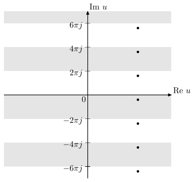
Figure 9.10: Periods of the preimage of the representation . Each strip (where there is no difference between gray and white strips) denotes a preimage of the entire complex plane with the exception of zero. The preimages denoted by the dots are preimages of one and the same value.
A multiplication by an integer in the preimage domain expands one period to periods . Respectively the function takes each value times as goes across all possible values in . Conversely, a division by an integer shrinks periods to one period and a previously single value of turns into different values of . This is another possible way to explain the fact that the equation has different solutions. Fig. 9.11 demonstrates the result of transformation of all preimages in Fig. 9.10 by a division by 2 corresponding to the equation . Notice that the preimages in Fig. 9.11 correspond to two different representation values, while the peimages in Fig. 9.10 were corresponding to one and the same representation value.
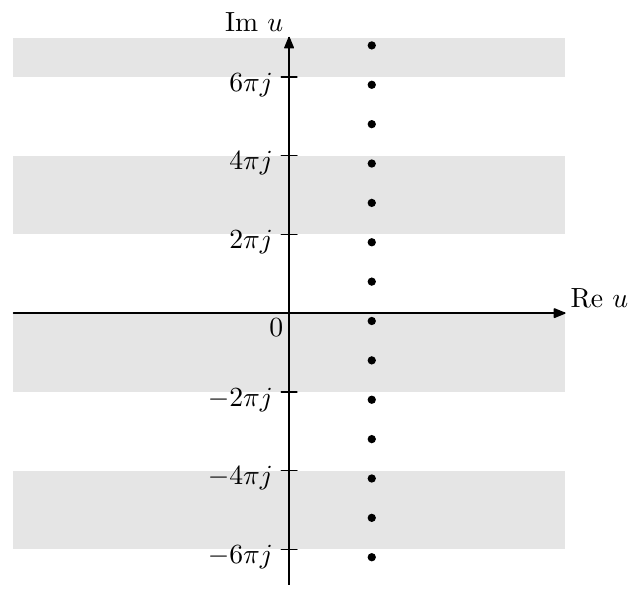
Figure 9.11: Transformation of the preimage points in Fig. 9.10 by division by 2.
The preimage of the real axis consists of two “horizontal” lines and , or, more precisely, of their periodic repetitions and , where . The line (and its repetitions) corresponds to the positive real numbers, the line (and its repetitions) corresponds to the negative real numbers. The preimage of the zero exists only in the limiting sense . Thus the multiplication of by is mapping the preimage of the real axis onto itself, therefore this multiplication’s representation maps the real axis onto itself.
The “vertical” lines are preimages of circles of radius , where moving upwards along such lines corresponds to the counterclockwise movement along the respective circle (Fig. 9.12), Particularly the imaginary axis is the preimage of the unit circle (note that a section of such line extending over a single imaginary period is sufficient to generate all possible values on such circle). Multiplication by maps the imaginary axis onto itself, thereby its representation maps the unit circle onto itself. A single preimage period is thereby mapped to periods , which corresponds to the unit circle being mapped to itself “ times”. We will shortly see that the mapping of the unit circle onto itself is the reason for the Butterworth poles being located on the unit circle.
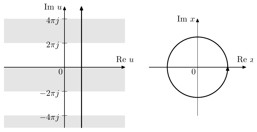
Figure 9.12: A circular trajectory and its preimage.
Even/odd poles
The poles of (9.18) are given by , which can be rewritten as . In the Butterworth case the solutions of were interleaved on the unit circle and also corresponded to even and odd values of in the solution formula for , where was defining the even poles and was defining the odd poles.
We will take effort to keep the same correspondence between the equations and the even/odd values of for other functions . In that regard it is instructive to first review the Butterworth case, but now using the just introduced linear scaling representation form, as it will then nicely generalize to other that we are going to use.
Let move along the unit circle in the counterclockwise direction. Its preimage defined by will respectively move upwards along the imaginary axis and so will . Respectively moves along the unit circle in the counterclockwise direction, just times faster, so while completes one circle, will complete only -th of a circle. The value of will be passing through the points and , since they are lying on the unit circle. At these moments the value of will be the solution of the equations and respectively (Figs. 9.13 and 9.14). There will be no other solutions since if moves in a circle of any other radius, this circle will map to a circle of a non-unit radius and will not go through the points . Thus Fig. 9.14 contains the full set of Butterworth poles, where the interleaving of the white/black dots on the circle in Fig. 9.14 arises from the interleaving of the white/black dots on the circular tajectory in Fig. 9.13.
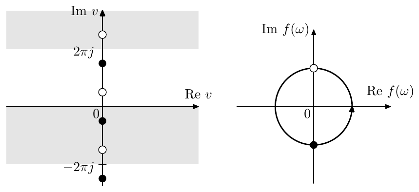
Figure 9.13: moving in a unit-radius circular trajectory, the points and their preimages.
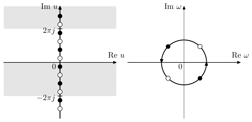
Figure 9.14: Transformation of Fig. 9.13 by (for ). The white and black dots on the circle are even/odd Butterworth poles in terms of .
Apparently, the passing of through corresponds to
where occurs at even and occurs at odd . The value of at these moments is
and the value of is
which is pretty much the same as the expression (8.13) we have developed before. The even/odd values of still correspond to the solutions of and respectively and thus we have a constency in referring to the solutions of as even poles and to the solutions of as odd poles.
Lowpass, bandpass and highpass filters
If we want in (9.18) to be a (unit cutoff) lowpass filter, then we should impose some additional requirements on :
where around the absolute magnitude of should smoothly grow from 0 to . Apparently the Butterworth filter’s function satisfies these requirements.
Similarly to Butterworth filter, with other filter types arising from (9.18) we will not be constructing which give a highpass or bandpass response. Instead, highpass and bandpass filters can be simply obtained by LP to HP and LP to BP substitutions respectively.
9.5 Trigonometric functions on complex plane
The trigonometric functions, such as , , and so on can be evaluated for complex argument values. In that regard they occur to be closely related to the hyperbolic functions , , and so on. The extention to can be obtained by simply evaluating the formulas
etc., where the function is allowed to take complex argument values. Notice that thereby we immediately obtain the “imaginary argument properties”:
etc., where intuitively we assume , but the formulas also work for .
By direct evaluation one could verify that all basic properties and fundamental trigonometric and hyperbolic identities continue to hold in complex domain. Particularly
etc. Also, apparently, conjugation commutes with the respective functions:
etc.
A direct corollary of (9.28) and the trigonometric formulas for the sum of arguments are the formulas allowing to express a trigonometric function a complex argument via the real and imaginary parts of the argument. E.g.
etc.
Periodicity
Since the periodicity property is retained in the complex domain, the former real periods of the trigonometric functions turn into strips on the complex plane. E.g. the periods of are shown in Fig. 9.15.
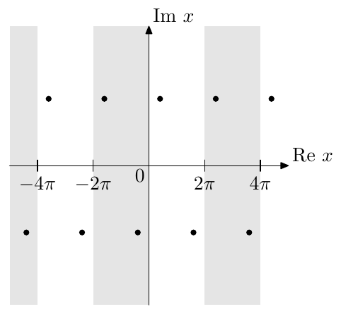
Figure 9.15: Periods of in the complex plane. All dots are preimages of one and the same value.
Due to the even symmetry of the cosine, almost every value occurs twice on a period (as illustrated by the dots in Fig. 9.15). That is if the value occurs at (that is ), then also occurs at . The exceptions are being and , which are mapped to themselves by if the periodicity of is taken into account.
Inverse functions
Inverting (9.22) and (9.23) we obtain
The principal value of the complex square root is defined as
where ,4 in which case thereby (9.30) is a generalization of arithmetric square root of real argument to complex domain. Notice that (9.30) gives the values on the upper imaginary semiaxis for real (provided for ).
The principal value of is defined in the usual way:
Respectively we can introduce the principal values of and as:
where we chose the signs in front of the square roots in such as way as to ensure that and .
The formulas (9.31a), (9.31b) raise concerns of numerical robustness in cases where the two terms under the logarithm sign are nearly opposite. By reciprocating the values under the logarithm signs we can rewrite them equivalently as
where the choice between (9.31a), (9.31b) and (9.31c), (9.31d) should be made based on comparing the complex arguments of the two terms under the logarithm sign. We should choose the formulas where we are adding two numbers whose complex arguments are not further than apart. Particularly, for real we may write
whereas the formula (9.31a) already works well for real .
Using (9.28) we can construct the principal values:
However besides the precision issues there are issues related to the principal values of switching leaf on the negative real axis. Technically this means that there is a discontinuity in the principal values of and on the negative real axis. With (9.31) this was generally tolerable, as the discontinuities weren’t arising for the “usual” values of the argument, which are for and for , since neither the argument of the square root nor the argument of the logarithm become real negative in such cases. With (9.32a), on the other hand, we do have a negative expression under the square root for real , which is the most important argument range.
We could therefore adjust (9.32a) to
The formulas (9.32b) and (9.32c) work well for , particularly precision-wise it doesn’t matter which of the two options in (9.32b) and (9.32c) are taken for , however they exibit a discontinuity for real . On the other hand, for purely imaginary argument values the formula (9.32b) can be rewritten essentially as (9.31e) to automatically choose the best option precision-wise:
Preimages of the real line with respect to
By (9.29a) attains purely real values iff or where . However, due to periodicity and evenness properties, each value is attained infinitely many times. We would like to choose a principal preimage of the real line with respect to . That is, we are interested in a (preferably continuous) minimal set of points, whose image under transformation is .
Note, that we do not really have to choose this principal preimage, as the discussions where we are going to refer to it should lead to exactly the same results no matter which of the preimages of the real line is taken. However, for the sake of clarity of discussion it is convenient to have an unambiguous reference preimage.
Apparently there are infinitely many choice possibilities, among which there are at least several “reasonable” ones. For the purposes of this text we will choose the principal preimage as shown in Fig. 9.16. The same figure also shows the periodic repetitions of the principal preimage.5
This principal preimage of the real axis thereby consists of three parts:
Apparently the principal preimage alone doesn’t cover all preimage points of the real line. Neither does it if we add its periodic repetitions in Fig. 9.16, since the lower-semiplane points of lines are still not included. We can include them by simply rotating all preimages in Fig. 9.16 around the origin, which corresponds to multiplication of all points by . Notice that by adding periodic repetitions we addressed the periodicity of , while by adding the preimages multiplied by we addressed the evenness property of .
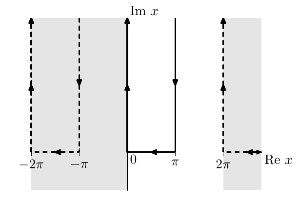
Figure 9.16: The principal preimage (solid line) of the real axis, with respect to , and its periodic repetitions (dashed lines).
Representations of horizontal preimage lines by
Equation (9.29a) implies that if the imaginary part is fixed and the real part is varying, that is the argument of the cosine is moving in a line parallel to the real axis, then the value of is moving along an ellipse in the complex plane, the real semiaxis of the ellipse being equal to and the imaginary semiaxis being equal to . Fig. 9.17 illustrates. At the real semiaxis is 1 and the imaginary semiaxis is zero. As grows both semiaxes grow, the imaginary semiaxis staying smaller than the real one in absolute magnitude (Fig. 9.18). Both semiaxes become equal in the limit where the ellipse turns into a circle.
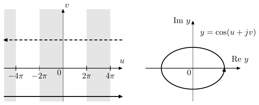
Figure 9.17: An elliptic trajectory and two its preimages. The picture is qualitative. In reality, for this kind of ellipse proportions the preimages would need to be located much closer to the real line.
Given and increasing , the movement of the point along the ellipse will be in the negative (clockwise) direction, due to the sign in front of the imaginary part in (9.29a). Respectively the positive (counterclockwise) direction movement will occur either for a decreasing or for a negative , where the latter is illustrated in Fig. 9.17.
The even symmetry of the cosine () implies that for each horizontal trajectory of the cosine’s argument, there is a symmetric trajectory which produces exactly the same cosine trajectory. This other trajectory is shown in Fig. 9.17 by the dashed line. Notice how this is related to the fact that flipping the sign of flips the direction of the movement along the ellipse: flipping the sign of is the same as flipping the sign of the entire cosine’s argument (that is flipping the signs of both and ), which leaves the elliptic trajectory unaffected, and then flipping the sign of , which reverts the direction of movement of both and .
From the fact that the semiaxes of the ellipse are and and therefore their absolute magnitudes are monotonically growing with (as one can see in Fig. 9.18) we can deduce that ellipses corresponding to different do not overlap, except for a switch from to , which simply changes the direction of the movement along the ellipse. That is for a given ellipse with and semiaxes there are only two preimages, as shown in Fig. 9.17. An exception occurs when the imaginary semiaxis of the ellipse is zero, in which case there is only one preimage, which is the real line.
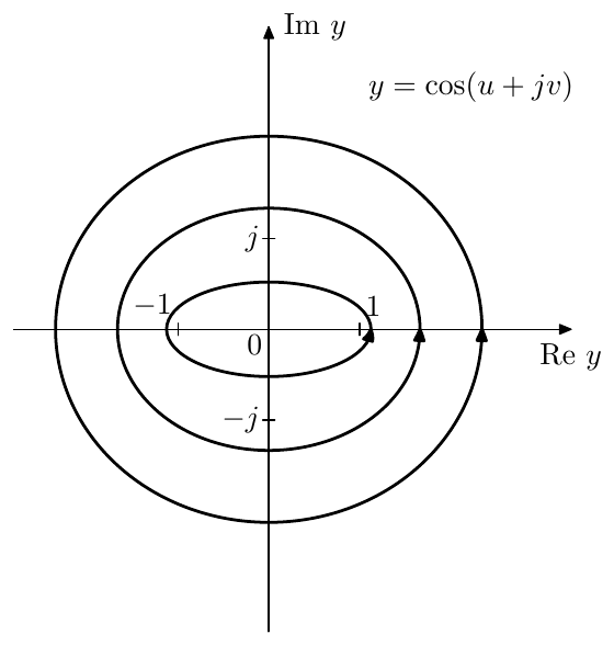
Figure 9.18: A family of elliptic trajectories generated from horizontal preimages .
Representations of horizontal preimage lines by
The secant function is obviously -periodic. In fact it bears quite a few further similarities to , which are easier to see if we write it in the polar form:
Consider a horizontal line (where is varying and ) and its respective representation . According to (9.33), moves in an ellipse-like curve around the origin, as shown in Fig. 9.19. At smaller magnitudes of the curve begins to look more like a figure of 8 (Fig. 9.20). The curve is not an ellipse anymore due to the reciprocation in (9.33a). On the other hand, by (9.33b) the “angular velocity” is the same as with , except that is has the opposite sign, therefore the rotation is happening in the opposite direction. Therefore for an increasing we get counterclockwise rotation iff rather than iff .
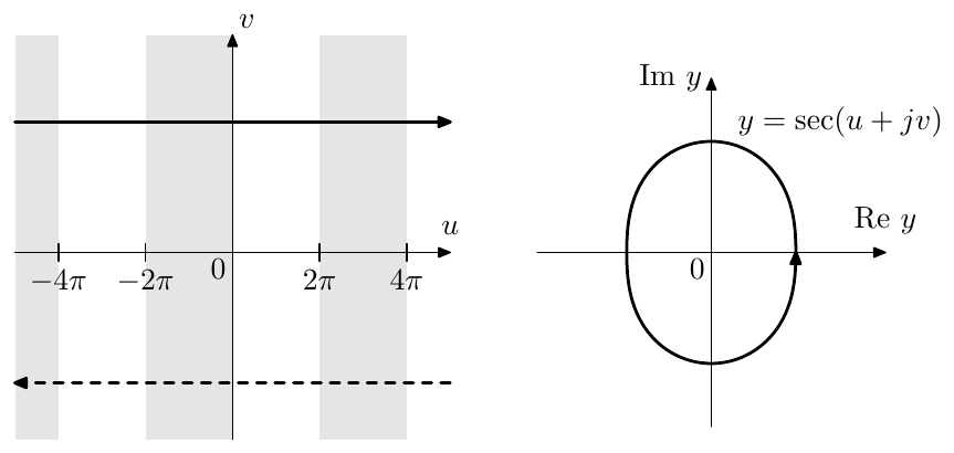
Figure 9.19: A quasielliptic trajectory and two its preimages (qualitatively).
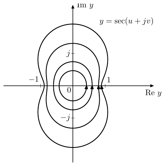
Figure 9.20: A family of quasielliptic trajectories generated from horizontal preimages .
9.6 Chebyshev polynomials
An -th order Chebyshev polynomial is defined as:
Fig. 9.21 illustrates. Notice the bipolar oscillations of equal amplitude (referred to as equiripples) on the range . As one can see in Fig. 9.21, the equiripple amplitude is unity.
Somewhat surprisingly, (9.34) can be equivalently written as an -th order real polynomial of at any , e.g. for we have , which is why they are called polynomials.
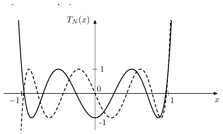
Figure 9.21: Chebyshev polynomials of even (solid) and odd (dashed) orders.
Note that takes complex values for and . We will also often assume taking complex values, therefore and will be complex as well. For even though becomes complex, the value is still real, and so is the polynomial itself.
A proper discussion of Chebyshev polynomials falls outside the scope of the book, as the respective information can be easily found elsewhere. Here we shall concentrate on the details which will be important for our purposes.
Chebyshev polynomials as representations of linear scaling
Introducing auxiliary variables and we rewrite (9.34) as
or, in the implicit form:
Thus the function is a representation of the linear scaling , the mapping function being . Note that by multiplying the whole preimage domain by we obtain a different (but equivalent) representation:
which gives us another equivalent expression for (9.34)
and its respective implicit form
In our discussion we will stick to using the cosine-based representation. The readers may draw parallels to the hyperbolic cosine-based representation if they wish.
In case of Butterworth filter-generating functions represented via mapping, the preimages were -periodic. This time they are -periodic. Additionally there is an even symmetry: and are preimages of the same .
Considering the effect the linear scaling on the principal preimage of the real line shown in Fig. 9.16, we obtain the following:
- The principal real half-period is expanded to to , which is responsible for the occurrence of the equiripples on the segment . Since is integer, other real half-periods expand similarly, without generating yet more representation values of . Thus is a single-valued function.
- The principal preimage of maps onto itself. The non-principal preimages of map onto some other preimages of . Similar mappings occur for the preimages of located in the lower complex semiplane. Thus is mapped by onto itself, corresponding to the monotonically growing behavior of for .
- The principal preimage of is mapped onto , which is a preimage of is is even and of if is odd. The non-principal preimages of (both those in the upper complex semiplane and in the lower complex semiplane) are mapped similarly. Thus is mapped by onto itself if is odd, or onto if is even, corresponding to the monotonic behavior of for .
Notice that these results correspond to the graphs in Fig. 9.21.
Now consider a line (where is some real constant value) parallel to the real axis in the preimage domain. Such lines are are, as we know from the previous discussion of the cosine of complex argument, the preimages of ellipses of various sizes, where the size grows with (Fig. 9.18). These ellipses are also not overlapping each other, except that the ellipses corresponding to and are identical (but have opposite orientations). Therefore maps any ellipse from this family onto another ellipse from this family and vice versa, similarly to how mapped the unit circle onto itself and mapped circles onto other circles. This time, however, the ellipse which is mapped onto itself, is the one with a zero imaginary semiaxis.
Notice that since the line is mapped to , the line stays in the same (upper or lower) semiplane after such mapping and goes in the same (to the right or to the left) direction. Thus, if is moving in an ellipse in a counterclockwise or respectively clockwise direction, then moves in the same direction.
Even/odd property
Since , a negation of corresponds to a shift of its preimage by . Respectively is shifted by , which will result in a negation of if is odd and will not change is is even. Therefore is even/odd if is even/odd:
Values at special points
The principal preimage of is . Therefore and . Therefore
By (9.37)
The principal preimage of is . Respectively and
where is a way of writing the sequence in the same way how is a way of writing the sequence .
Leading coefficient
Knowing that is a real polynomial of order , we can obtain its leading coefficient by evaluating the limit
For the purposes of this book’s material, we won’t need to be able to explicitly find the other coefficients and will therefore skip this topic.
Zeros
Rather than being interested in the values of the coefficients of Chebyshev polynomials, for our purposes it will be more practical to know the locations of their zeros. Letting we have
Respectively
and
which means that the zeros are
where there are distinct values corresponding to . Notice that the zeros are all real and lie within . Also notice that , therefore the zeros are positioned symmetrically around the origin. Consequently, if is odd, one of will be at the origin.
Using (9.38) we can write in the factored form:
where we are taking the product only over the positive zeros using the symmetry of the zeros relatively to the origin, and the odd factor (where denotes bitwise conjunction) appears only for odd where one of the zeros is at the origin. The normalizations by are simply appearing from the requirement that each factor must be equal to 1 at , so that .
Renormalized Chebyshev polynomials
The factored form (9.39) offers some nice insights into the comparison of the behavior of and . Writing is a comparable factored form we have
where “taking the product over ” means that we are having as many factors as there are positive zeros in the Chebyshev polynomial . Thus the difference between and is that the factors are replaced by .
Apparently, if then and respectively (9.39) is approaching . Unfortunately we cannot express this as simply , since the zeros of are fixed.
To mathematically express this variation of zeros, we can notice that the value of (9.39) at is always unity. Therefore we can introduce the polynomials
to which we refer as renormalized Chebyshev polynomials. By construction , while the zeros of are . Therefore
and
The formula (9.41) cannot be evaluated for , however we apparently can take the limit at as the value of and thus
Notice that the formula (9.42) perfectly works at .
Since the equiripple amplitude of is unity, by (9.41) the equiripple amplitude of is . The equiripple range of is respectively transformed into the equiripple range of . Thus simultaneously controls the equiripple amplitude and the equiripple range of (Fig. 9.22).
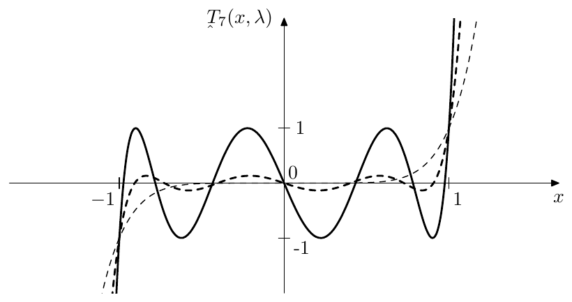
Figure 9.22: Renormalized Chebyshev polynomial for (solid), (dashed) and (thin dashed).
As we won’t need , we won’t consider that option. As for the large values of , it will be practical to restrict the value of so that . Apparently this means where . Notice that since , it follows that .
Often it will be even more practical to restrict to . At the equiripple amplitude of is already unity. As grows further the equiripple amplitude quickly grows, reaching at . Also the equiripple range exceeds , which could become inconvenient for our purposes.
In order to simplify the notation, often we will omit the parameter, understanding it implicitly, and simply write instead of .
Slope at
Let’s compare the factors of (9.42) and (9.40). Computing the differences:
and taking into account that , we notice that for and the differences (9.43) are strictly positive and respectively the factors of (9.42) are larger than those of (9.40). In the range , since all factors are positive, we have
By the even/odd symmetries of and :
From (9.43) we can also notice that the difference grows with , thus at larger the polynomial exceeds (in absolute magnitude) by a larger amount.
At we have . For this specific case we would like to get a more exact estimation of the steepness of the slope at , to get an idea of how much steeper is the slope of compared to . We have already seen that the leading coefficient of is , which means that at the polynomial grows times faster than . It would be also informative to compare their slope at .
An attempt to compute the derivative of at in a straightforward manner results in an uncertainty, thus it’s easier to take a way around. At points infinitely close to we expand the cosine into Taylor series up to the second order term:
This scaling by times in the preimage domain () corresponds to scaling by times in the representation domain () and we obtain
On the other hand
Thus at Chebyshev polynomials grow times faster than .
9.7 Chebyshev type I filters
Chebyshev (or, more precisely, Chebyshev type I) filters arise by using renormalized Chebyshev polynomials as in (9.18).6 The main motivation to use renormalized Chebyshev polynomials instead of (which is used in Butterworth filters) is that, as we already know they grow faster than for , which results in a steeper transition band compared to Butterworth filters. The tradeoff is that in order to achieve a steeper transition band we need to allow ripples in the passband. At the same time, the analytical expressions (9.34) and (9.36) allow to easily obtain the function inversion of the polynomial, allowing analytical computation of the filter’s internal variables (such as pole positions) for arbitrarily high polynomial orders , which would have been impossible for polynomials of a fully general form.
Thus, in (9.18) we let
that is
The parameter of is affecting the equiripple amplitude of and thereby the equiripple amplitude in the passband of . It is convenient to introduce the additional variable
which is simply equal to the equiripple amplitude of . Using (9.44) we particularly may write
Notice that (9.44) allows to compute from and vice versa. Therefore, if we are given a desired equiripple band , we thereby have specified and can use (9.44) to compute . Conversely, if we are given a desired equiripple amplitude (which is a more common case), we thereby have specified and can invert (9.44) to compute :
(where denotes the inverted function ).
The amplitude response is thus varying within on the equiripple range . On the other hand, (or, equivalently, ) affects the slope of (and respectively the slope of ) at . The slope steepness is thereby traded against the equiripple amplitude, where steeper slopes are achieved at larger equiripple amplitudes. Fig. 9.23 illustrates.
Poles of Chebyshev type I filters
We have mentioned that the (9.34) is actually a polynomial of . Therefore the denominator of (9.18) is a polynomial of and we can find the roots of this polynomial, which are simultaneously the poles of . The equation for these poles is thus
or
or
or, introducing
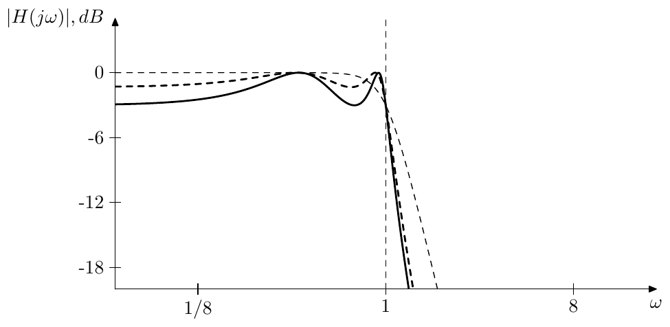
Figure 9.23: Chebyshev type I filter’s amplitude responses for and (solid), (dashed) and (Butterworth, thin dashed).
It is quite helpful to use the interpretation of in terms of representation preimage domain to solve (9.45). Recall that maps ellipses (of a special ellipse family, where the real and imaginary semiaxes and are related as , so that they can be represented as , for some ) to ellipses (of the same family). In the preimage domain these ellipses correspond to lines parallel to the real axis.
Suppose is moving in such an ellipse. This corresponds to its preimages moving along two lines . Let be one of the preimages in , to which we will refer as the principal preimage. Respectively the full family of preimages is . The principal preimage of is therefore , moving along the line . The full family of preimages of is respectively and is moving along the lines . Therefore is moving in an ellipse whose real and imaginary semiaxes are and respectively.
We wish to move in a counterclockwise direction along an ellipse which goes through the points. Then at the moments when we will obtain solutions of (9.45). We additionally wish the real part of the preimage of to be increasing during such movement,7 therefore for a counterclockwise movement of we need . Therefore, in order for the ellipse to go through , the imaginary semiaxis of this ellipse must be equal to and thus we obtain:
According to (9.29a), the purely imaginary values of a cosine are attained when the real part of the cosine’s argument is equal to , where . Thus, the values will be attained by at
where, since , the value is attained at and other even values of . Thus, the solutions of the even pole equation will occur at even values of . Fig. 9.24 illustrates.
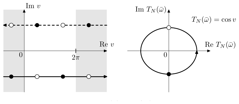
Figure 9.24: Preimages of (qualitatively, the scales of the real and imaginary axes in the plane are not equal).
From (9.46) we obtain
where there are essentially different preimages of occuring at consecutive values of all lying on the line . Going back to the representation domain we obtain lying on the respective ellipse:
Fig. 9.25 illustrates.
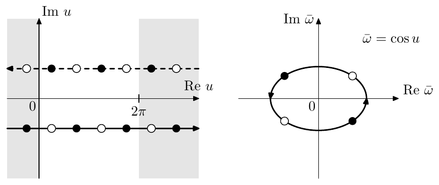
Figure 9.25: Transformation of Fig. 9.24 by (for ). The white and black dots on the ellipse are even/odd Chebyshev poles in terms of . (The picture is qualitative, as the scales of the real and imaginary axes in the plane are not equal.)
Switching to we have:
Note that formally allowing to take real values and letting we obtain and which is a real positive value. Since the imaginary part of the cosine’s argument is negative, the values of are moving counterclockwise for increasing , starting from the value on the positive real semiaxis occuring at . That is, the values of are moving counterclockwise starting from the positive real semiaxis. As we already found out, the values occurring at even/odd correspond to even/odd poles respectively, and thus the even and odd poles are interleaved on the ellipse.
Switching from to we obtain the expression for the poles:
Since the values of are moving counterclockwise starting from the real positive semiaxis, the values of are moving counterclockwise starting from the imaginary “positive” semiaxis, which means that starting at we first obtain the stable poles at . The next values of will give the unstable poles.
Note that since never takes integer values, the real part of is never zero and there are no poles on the imaginary axis. The poles are also symmetric relatively to the real and imaginary axes and we can discard the half of the poles located in the right complex semiplane in the same way how we did it with the Butterworth filter. Figs. 9.26 and 9.27 illustrate.8
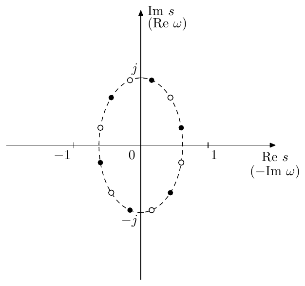
Figure 9.26: Chebyshev type I filter’s even (white) and odd (black) poles for (including the poles of ).
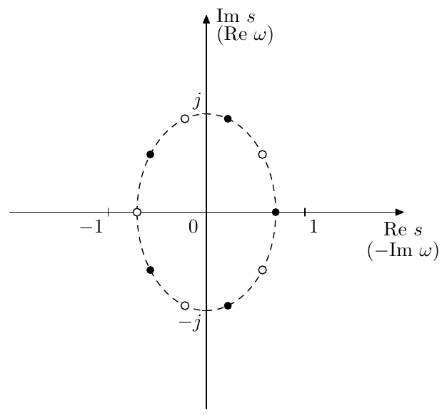
Figure 9.27: Chebyshev type I filter’s even (white) and odd (black) poles for (including the poles of ).
In Figs. 9.26 and 9.27 one could notice that the poles are condensed close to the imaginary axis while the Butterworth poles were evenly spacing. This is easily explained in terms of (9.29a), which gives
Now, if had been equal to 1, we would have had , which would have resulted in an even angular distribution of poles. However, since , the poles are located closer to the real axis in the plane or closer to the imaginary axis in the plane.
Gain adjustments
Having obtained the poles and keeping in mind that there are no zeros, we can obtain the transfer function in the form
where the gain could be obtained by evaluating the above product at and comparing to . It could be a bit more practical though, to write as a product of 1-pole lowpasses with unity passband gains:
where are the (possibly complex) cutoffs and where the coefficient is different than in the previous formula. For (9.50) we are having and thus, using (9.18), we can obtain from
Another option is to obtain the leading gain from the requirement arising from
However this might accidentally result in a phase response at , (since we used rather than as a reference) therefore one needs to be careful in this regard.
Using the default normalization of the Chebyshev filter’s gain given by (9.51), we obtain the amplitude response varying within on the range . We could choose some other normalizations, though. E.g. we could require , which will be automatically achieved if we simply let in (9.50). Or we could require the ripples to be symmetric relatively to the zero decibel level, which is achieved by multiplying (9.51) by :
so that varies within within the equiripple band.
Butterworth limit
Since at we have , in the limit Chebyshev type I filter turns into a Butterworth filter of the same order .
Simultaneously the ellipse semiaxes and in (9.49) are both approaching the unity length. Indeed, letting (which is equivalent to ), we have
Thus and are asymptotically identical and therefore . In a similar way we can show that .
9.8 Chebyshev type II filters
Chebyshev polynomials have equiripple behavior on and grow to infinity outside of that range. By reciprocating the argument: , we obtain equiripple behavior on and infinite growth for . By further reciprocating the value of the polynomial: , we have again small values on the range , while for the polynomial’s value exhibits equiripple oscillations around infinity. We therefore introduce the function
where Fig. 9.28 illustrates the behavior of . We will refer to as a double-reciprocated (once in argument and once in value) Chebyshev polynomial.
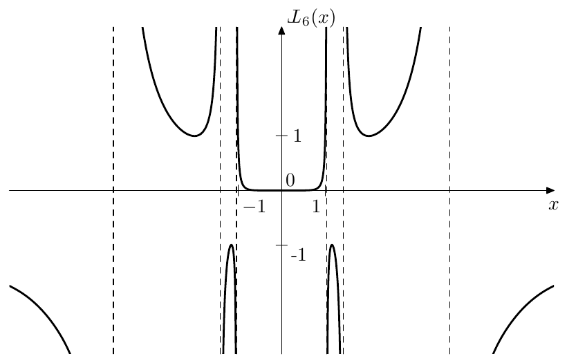
Figure 9.28: Double-reciprocated Chebyshev polynomial .
The equiripple oscillations around infinity are also better visible in the arctangent scale (Fig. 9.29). More specifically, on and the value oscillates between and , never becoming less than 1 in the absolute magnitude. We could refer to that fact by saying that the amplitude of these oscillations around is unity, thereby taking the minimum absolute magnitude of the oscillating value as the oscillation amplitude, even though that might be considered some kind of a misnomer. We will be using this definition of amplitude of oscillations around infinity further in the text.
We also introduce the renormalized version of the double-reciprocated Chebyshev polynomials by double-reciprocating :
where we have . Notice that we didn’t reciprocate the parameter. The idea is that and that
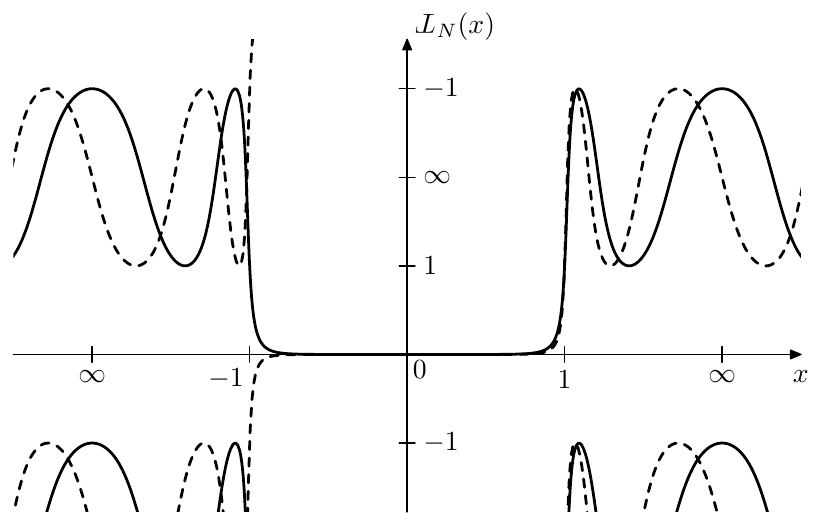
Figure 9.29: Double-reciprocated Chebyshev polynomials of even (solid) and odd (dashed) orders, using arctangent scale in both axes.
Fig. 9.30 illustrates. As usual, we will often omit the parameter, understanding it implicitly.
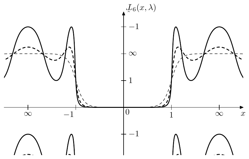
Figure 9.30: Renormalized double-reciprocated Chebyshev polynomial for (solid), (dashed) and (thin dashed).
By (9.52) the amplitude of the equiripples of is . By using the same equation (9.44) as we have been using for Chebyshev type II filters we have , that is the equiripple amplitude is . This is actually a convenient notation, since in this case we are having smaller (closer to ) equiripples at smaller . We also thereby have:
By writing the Chebyshev polynomial as a polynomial:
we find that the double-reciprocated Chebyshev polynomial is a rational function of :
The same apparently is true for and therefore we could try using as in (9.18).
Letting in (9.18) we obtain a Chebyshev type II filter, this time trading the ripples in the stopband against the transition band’s rolloff (Fig. 9.31). The stopband peaks are achieved at , thus the ripple amplitude is .
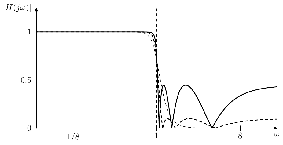
Figure 9.31: Chebyshev type II filter’s amplitude responses for and (solid), (dashed) and (Butterworth, thin dashed). Notice the usage of the linear amplitude scale, which is chosen in order to be able to show the amplitude response zeros.
as representations of linear scaling
In order to find the poles of a Chebyshev type II filter we are going, as usual, to interpret the function as a representation of the linear scaling . This time we need the following mapping:
Same as with , the multiplication by expands the principal real period to and there are similar transformations of the preimages of the real axis. The transformations of quasielliptic curves (shown in Fig. 9.20) which are representations of horizontal lines in the preimage domain are also occurring in a similar fashion, each such curve being transformed into another such curve.
Poles of Chebyshev type II filters
The pole equation is
The even/odd pole equations are respectively
or
or, introducing
where the “+” sign corresponds to the even poles and the “-” sign to odd poles.
Suppose is moving in a counterclockwise direction in a quasielliptic curve which is a representation of (where, according to our previous discussion of the properties of the mapping, ). This results in a similar counterclockwise motion of . We wish to pass through the points going counterclockwise.
At this point we could follow similar steps as we did for Chebyshev type I filters, using the preimage linear scaling interpretation of to obtain the points where . However we also could notice that . Therefore we could reuse the results of our discussion of Chebyshev type I filters, where we needed to go clockwise through . That is, we need the value of to move in the same trajectory going through the same points as in the Chebyshev type I case, just in the opposite direction. This can be achieved by flipping its preimage line from the lower semiplane to the upper semiplane. Therefore the values of passing through going clockwise should occur at and thus
The other difference to the case of Chebyshev type I filters is that the argument of is rather than . Therefore we need to replace in (9.47) with obtaining
and
Since , we have and thus
The poles of Chebyshev type II filters are therefore negated reciprocals of the poles of Chebyshev type I filters.9 By the interpretation of as linear scaling in the preimage domain, Chebyshev type II poles should lie on quasielliptic trajectories, such as the ones shown in Fig. 9.19 and Fig. 9.20. Notice that, despite the negated reciprocation, the formula (9.53) still first gives the stable poles, due to the flipped sign of compared to (9.49).
Zeros of Chebyshev type II filters
According to our discussion in Section 9.4 of using rational , Chebyshev type II filters also should have zeros, which in terms of coincide with poles of . The zero equation is thereby
or
or, equivalently,
The solutions of (9.54) thereby obtained from the zeros of (given by (9.38)) by
or
or, in terms of
An additional consideration arises at odd where one of the values given by (9.38) occurs at the origin, which after the reciprocation gives the infinity. This means that there is no corresponding finite zero of and no corresponding factor in the numerator of . Respectively the order of the numerator of becomes 1 less than the order of the denominator. This automatically results in , that is has a zero at the infinity, as required by the reciprocation of the values given by (9.38). Fig. 9.32 provides an example.
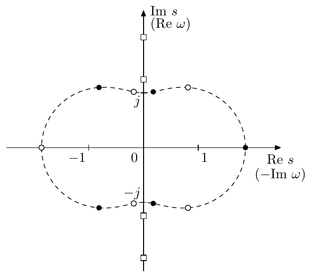
Figure 9.32: Poles (white and black dots) and zeros (white squares) of a Chebyshev type II filter of order . Each of the zeros is duplicated, but the duplicates are dropped together with the unstable poles.
Filter gain
Since there are no ripples in the passband, there is little reason to attempt any gain adjustments and the filter gain needs simply to be chosen from the requirement , thereby defining the leading gain coefficient of the cascade form (8.1).
Butterworth limit
Since in the limit Chebyshev type II filter turns into Butterworth filter.
Notice that the pole formula (9.53) is essentially the negated reciprocal of (9.49). On the other hand, negation and/or reciprocation turn Butteworth poles into themselves (if nonstable poles are included), therefore, since in the limit (9.49) gives Butterworth poles, (9.53) also does the same.
9.9 Jacobian elliptic functions
The next class of equiripple filters which we would like to introduce are elliptic filters. Chebyshev filters were based on the cosine function and required a wider spectrum of trigonometric and hyperbolic functions for their analysis. Similarly, elliptic filters are based on Jacobian elliptic cosine function and require other Jacobian elliptic functions for their analysis. Since Jacobian elliptic functions are not a part of widely spread common knowledge, on the contrary, the freely available resources are rather scarce, we are going to introduce them and discuss their properties relevant for this book’s material.
Additional information can be found in the reference texts listed at the end of this chapter. The results presented here and in the rest of this chapter without any kind of proof or justification are either taken directly or derived from these texts.
Elliptic integrals of the first kind
One of the most common ways to introduce Jacobian elliptic functions is as some kind of special inverses of the elliptic integral of the first kind, which we therefore will briefly discuss first.
The elliptic integral of the first kind is the function notated defined by the formula:
The parameter is referred to as elliptic modulus. Normally . At we simply have .
The value of at is often of a particular interest, which motivates the introduction of the complete elliptic integral of the first kind:
Respectively we are having
The graph of is shown in Fig. 9.33. Notice that grows with (which is obvious from (9.55)).
The elliptic modulus is sometimes expressed as where is referred to as the modular angle. Given a modular angle , often one also needs the complementary modular angle which is simply defined as
Respectively there is the complementary elliptic modulus:
and the complementary complete elliptic integral of the first kind:
Notice that decreases as increases and vice versa. On the other hand is a monotonically increasing function. Therefore the ratio monotonically decreases with growing . Fig. 9.34 illustrates, where we use the modular angle in the abscissa scale in order to make the symmetry between and explicitly visible.
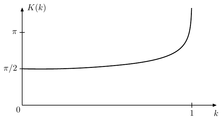
Figure 9.33: Complete elliptic integral of the first kind .
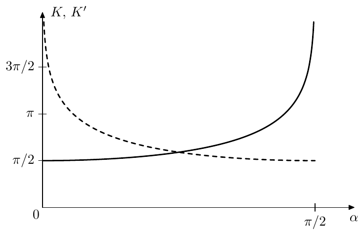
Figure 9.34: Complete elliptic integral of the first kind (solid line) and the complemetary complete elliptic integral of the first kind (dashed line), plotted against the modular angle .
Jacobian elliptic functions
There are 12 different Jacobian elliptic functions but we will concentrate only on 6 of them. The ones we introduce will bear strong similarities to certain trigonometric and/or hyperbolic functions, becoming equal to them in the limit.
We will define Jacobian elliptic functions in terms of the so called amplitude, which is defined as a function , which is the inverse of the elliptic integral of the first kind:
That is, for a given the function gives such that . Note that since in the limit we have , we are respectively having .
As with elliptic integral , the second argument serves a role of the function’s parameter, the “primary” argument of the function being . Often this parameter is simply omitted and understood implicitly: . Even more commonly, this is done for Jacobian elliptic functions (which are having exactly the same arguments as the amplitude).
Now, from the six Jacobian elliptic functions that we are going to introduce, the four of our primary interest will be:
-
Jacobian elliptic “sine” is defined by the equation
where . Or simply, .
Fig. 9.35 provides example graphs of , where we could also notice that is -periodic. The value is simply a short notation for the complete elliptic integral , evaluated for the same modulus which is used in . Please also note that the graphs in Fig. 9.35 are plotted “in terms of ”, that is different abscissa scales are used for different graphs in the same figure. This has been done in order to provide a better visual comparison of different with different periods.
Since the limit we have , the elliptic sine turns into into .
-
Jacobian elliptic “cosine”10 is defined by the equation:
where . Fig. 9.36 illustrates, where one could observe that is -periodic. Apparently .
-
Jacobian elliptic “tangent”/elliptic “hyperbolic sine” is defined by the equation:
where . Fig. 9.37 illustrates, where one could observe that is -periodic.
Apparently . However, the function also bears strong similarities to the hyperbolic sine, becoming equal to it in the limit . In this book we will be mostly using the similarity of to , therefore we will typically refer to as elliptic “hyperbolic sine”.
-
Jacobian elliptic “hyperbolic cosine” is defined by the equation:
where . Fig. 9.38 illustrates, where one could observe that is -periodic. This function becomes equal to in the limit .
We will also introduce two “auxiliary” functions:
-
Jacobian elliptic “cosecant” (Fig. 9.39)
-
Jacobian elliptic “secant” (Fig. 9.40).
Since these two are simply reciprocals of and , we won’t be discussing them much, however they will be used occasionally.
From the previous discussion we could conclude that is the common period of all six introduced elliptic functions (where the elliptic “trigonomet- ric” functions are -periodic and the elliptic “hyperbolic” functions are - periodic). For that reason is referred to as the quarter-period.
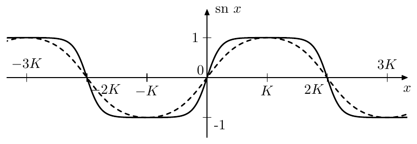
Figure 9.35: Jacobian elliptic sine for (dashed) and (solid).
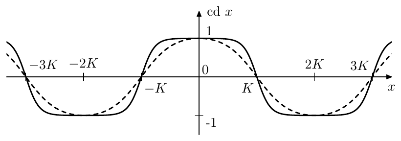
Figure 9.36: Jacobian elliptic cosine for (dashed) and (solid).
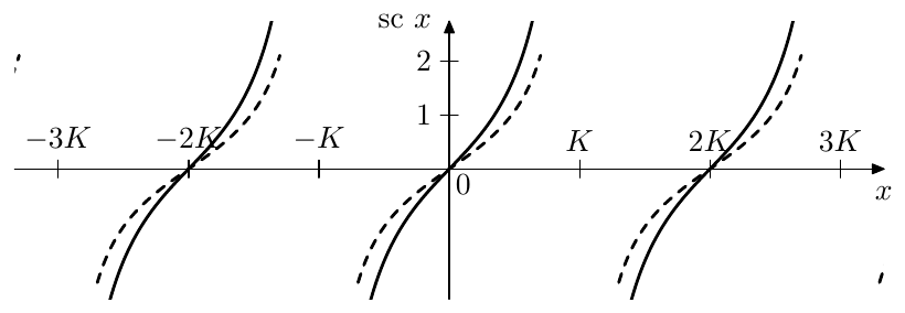
Figure 9.37: Jacobian elliptic “hyperbolic sine” (or “trigonometric tangent”) for (dashed) and (solid).
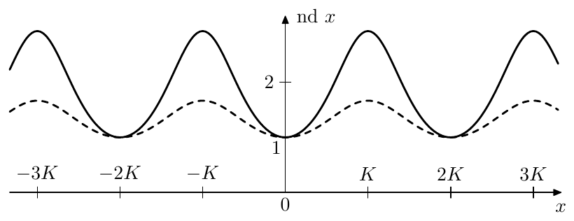
Figure 9.38: Jacobian elliptic “hyperbolic cosine” (dashed) and (solid). The maxima are at .
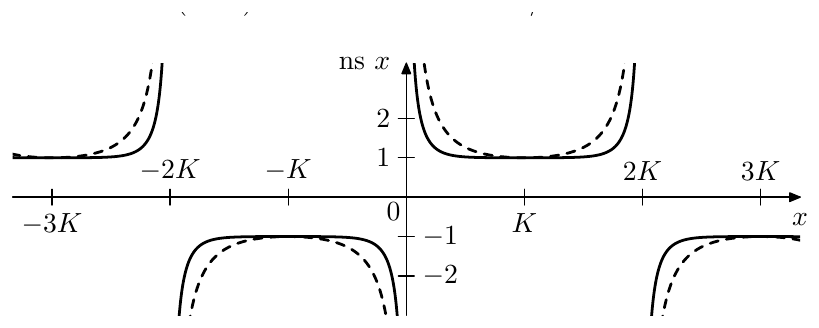
Figure 9.39: Jacobian elliptic cosecant (dashed) and (solid).
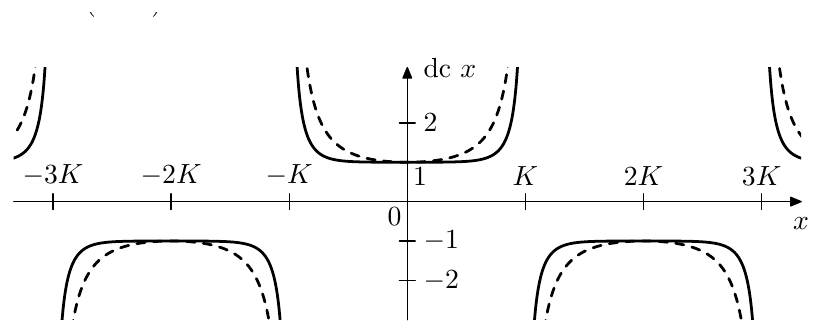
Figure 9.40: Jacobian elliptic secant (dashed) and (solid).
Complex argument
Jacobian elliptic functions can be generalized to complex argument values. Re- markably, all of the six introduced functions can be obtained from each other by shifts and/or rotations of the argument in the complex plane (with some possible scaling of the resulting function’s value).
Before discussing any Jacobian elliptic function on the complex plane we need to introduce the imaginary quarter period which is simply equal to the complementary complete elliptic integral: . Jacobian elliptic functions are also periodic in the imaginary direction, where the elliptic “trigonometric” functions are -periodic and the elliptic “hyperbolic” func- tions are -periodic, e.g. .
The real and imaginary quarter periods create a virtual grid on the complex plane (Fig. 9.41). We will be particularly interested in the values that Jacobian elliptic functions are taking along the lines of this grid.
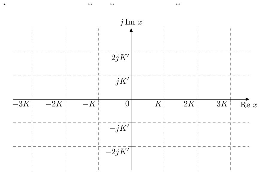
Figure 9.41: Quarter-period grid.
Let’s start with . It turns out that the values of on this grid are always equal to the (possibly scaled by some real or imaginary coefficient) values of one of the six introduced Jacobian functions evaluated for the real or the imaginary part of . Fig. 9.42 illustrates.
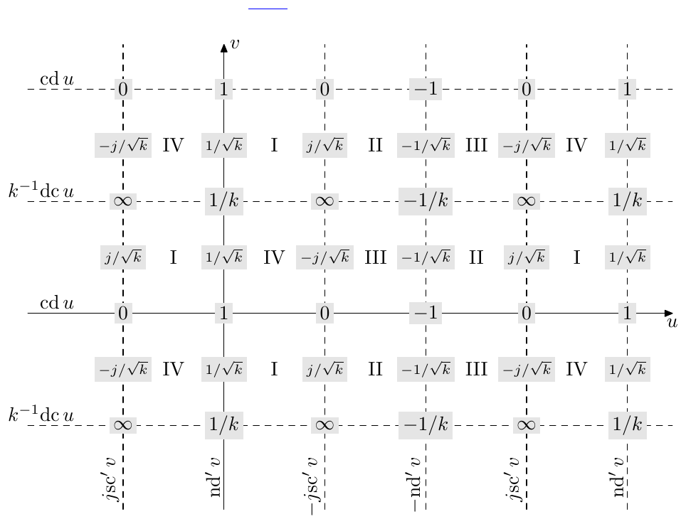
Figure 9.42: Values of on the quarter-period grid.
The expressions at the ends of the quarter-grid lines in Fig. 9.42 are what is equal to on each of these lines, where the notation is , . E.g. for the function’s value is . For the function’s value is , that is the primed notation denotes the usage of the complementary elliptic modulus. Apparently, the complementary modulus needs to be used for all grid lines parallel to the imaginary axis, since the quarter period in that direction is .
The roman numerals in the middle of the grid cells denote the complex quadrant to which the values of belong for inside the respective grid cell. The quadrants are numbered starting from the positive real semiaxis in the counterclockwise direction. Fig. 9.42 also shows the function values at the intersections of the grid lines. Additionally the values exactly in the middle between the horizontal grid lines are shown. E.g. . The readers are encouraged to compare the values listed in Fig. 9.42 to the graphs in Figs. 9.35 through 9.40.
Similarly to how the trigonometric sine is obtained from the trigonometric cosine by a shift by the quarter-period (which also holds for complex ar- guments), the Jacobian sine is obtained from the Jacobian cosine by a shift by the quarter period : . Respectively, the content of Fig. 9.42 becomes shifted by resulting in the picture in Fig. 9.43.
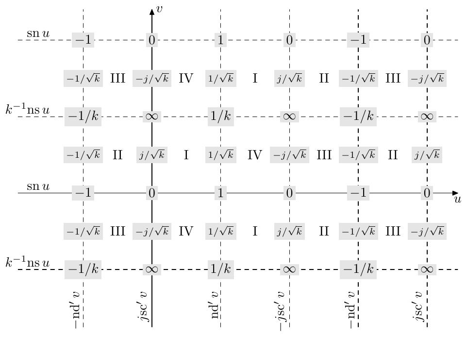
Figure 9.43: Values of on the quarter-period grid.
From Fig. 9.42 one could notice that . It turns out that this equality holds not only for real but for any complex . That is, Jacobian hyperbolic cosine can be obtained from Jacobian cosine by rotation of the complex plane by and swapping of and (which effectively swaps and ).11 Fig. 9.44 illustrates.
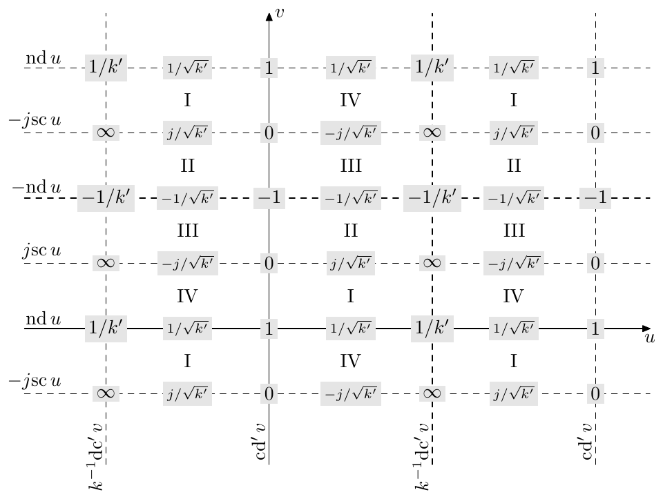
Figure 9.44: Values of on the quarter-period grid.
In a similar fashion, in Fig. 9.43 one could notice that . This equality also holds not only for real but for any complex . That is, Jacobian hyperbolic sine can be obtained from Jacobian sine by rotation of the complex plane by clockwise, swapping of and and dividing the result by (or, equivalently, multiplying by ). Alternatively, recalling that is obtained from by a shift by a real quarter period, we could have simply shifted the content of Fig. 9.44 downwards by an imaginary quarter period and divided it by . Fig. 9.45 illustrates.
The functions and are easily obtainable from Figs. 9.42 and 9.43 by a shift by one imaginary period (and a multiplication by ).
Properties of Jacobian elliptic functions
There are lots of analogies between trigonometric/hyperbolic and Jacobian ellip- tic functions including similarities between their shapes, which one can see from Figs. 9.35 through 9.40. We are going to list some of the properties of Jacobian elliptic functions comparing them against similar properties of their trigonomet- ric/hyperbolic counterparts, where possible. The value of the argument will be assumed complex, unless otherwise noted. It is highly recommended to refer to Figs. 9.35 through 9.40 and to Figs. 9.42 through 9.45 while studying the properties below.
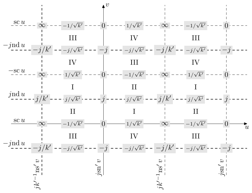
Figure 9.45: Values of on the quarter-period grid.
-
Reduction to trigonometric/hyperbolic functions at or :
-
The functions are analytic (except at their poles).
-
Real function values for real argument :
-
The functions commute with complex conjugation:
etc.
-
Odd/even symmetries
- Imaginary argument
where we intuitively assume , although the properties hold for any .
- Periodicity along real axis:
and along imaginary axis:
Note that the periodicity property of and along the imaginary axis is the dual of the periodicity property of and along the real axis, the duality arising from the imaginary argument property.
- Shift by function’s half-period12 in the real direction
and in the imaginary direction
- Shift by function’s quarter-period
- Symmetry around function’s quarter-period point (this follows from the odd/even symmetries and the shift by function’s half-period property) in the real direction:
and in the imaginary direction:
- Pythagorean theorem
(we won’t need the respective properties for the “hyperbolic” functions). There is another useful Pythagorean-like identity:
- Sum of arguments
(we won’t need the respective properties for the other functions).
- Complex argument
where , . This is a direct corollary of (9.70). One can use (9.71) to show that the values of on a single grid cell in Fig. 9.42 belong to one and the same complex quadrant.
- Logarithmic derivative
Periodicity
As we already mentioned, Jacobian elliptic functions are periodic in real and imaginary direction. E.g. is - and -periodic. Thus the periods of are rectangles in the complex plane, the horizontal dimension of each rectangle being equal to and the vertical dimension being equal to . Fig. 9.46 illustrates.
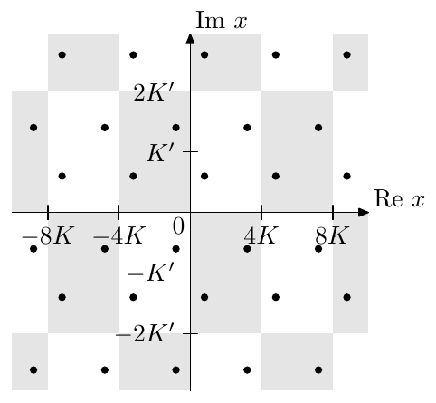
Figure 9.46: Periods of in the complex plane. All dots are preimages of one and the same value.
Due to the even symmetry of the elliptic cosine, almost every value occurs twice on a period (as illustrated by the dots in Fig. 9.46). That is if the value occurs at (that is ), then also occurs at . The exceptions are being and , which are mapped to themselves by if the periodicities of are taken into account.
Similar considerations apply to , and .
Preimages of the real line
By (9.71) attains purely real values iff or where , which is also illustrated by Fig. 9.42. Similarly to , we would like to choose a principal preimage of the real line with respect to the transformation . Since for , we would like the principal real line preimage for to approach to the respective principal preimage for as . Under this requirement there is only one choice, which is shown in Fig. 9.47.
This principal preimage of the real axis thereby consists of five parts:
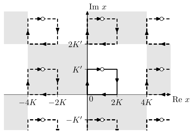
Figure 9.47: The principal preimage (solid line) of the real axis, with respect to , and its periodic repetitions (dashed lines).
where Fig. 9.42 can serve as additional reference.
The punctured point at in Fig. 9.47 corresponds to . In principle it can be included into the preimage if we consider the extended complex plane as the codomain of , in which case the preimage consists only of four parts:
where denotes a range on the real Riemann circle containing the infinity in its middle.
As with , the principal preimage alone doesn’t cover all preimage points of the real line. Neither does it if we add its periodic repetitions in Fig. 9.47, since we are covering only half of the entire length of each of the lines . We can cover the remaining halves by rotating all preimages in Fig. 9.47 around the origin, which corresponds to multiplication of all points by . Notice that by adding periodic repetitions we addressed the periodicity of , while by adding the preimages multiplied by we addressed the evenness property of .
9.10 Normalized Jacobian elliptic functions
In Fig. 9.42 we can observe that the “four building blocks” of the Jacobian cosine’s values on the quarter-period grid lines are , , , , and . Plotting these functions in the arctangent scale we obtain the picture in Fig. 9.48.
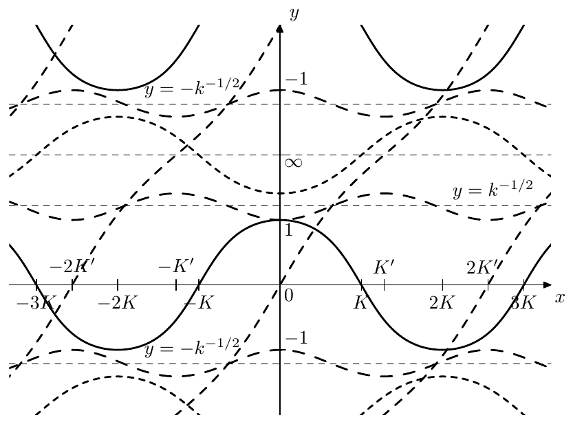
Figure 9.48: , , and .
The collection of the function graphs in Fig. 9.48 has obvious symmetries with respect to the horizontal lines and . It is also approximately symmetric with respect to (where, since , it follows that , so the line is located above ). This approximate symmetry obviously arises from the reciprocal symmetries due to (9.67):
(where (9.73c) is not due to (9.67) but simply follows from the definition of the function: ).
Therefore the centers of this reciprocal symmetry are at . By multiplying all functions plotted in Fig. 9.48 by we will shift the centers of the reciprocal symmetry to . Thus consideration motivates the introduction of normalized Jacobian elliptic functions
(note that for the “hyperbolic” functions we are using rather than for the normalization!). Thereby (9.73) become:
and Fig. 9.48 turns into Fig. 9.49.
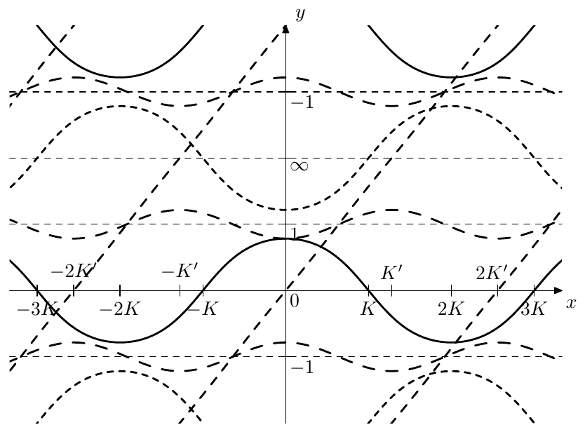
Figure 9.49: , , and .
Apparently, , , , , and are the building blocks of in the same way how , , , , and are the building blocks of . Fig. 9.50 illustrates. Notice that we don’t need non-unity scaling by anymore, only shifts, rotations and scaling by are required to convert between the respective functions. Fig. 9.51 provides a similar illustration for . The diagrams Fig. 9.43 and 9.45 are transformed in a similar way.
For normalized elliptic functions the reciprocal symmetries of (9.67) take the form
with the analogous shift properties (9.65) taking the form
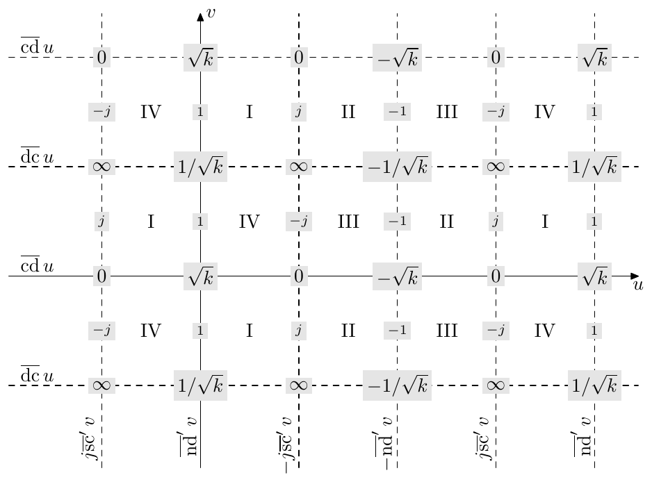
Figure 9.50: Values of on the quarter-period grid (compare to Fig. 9.42).
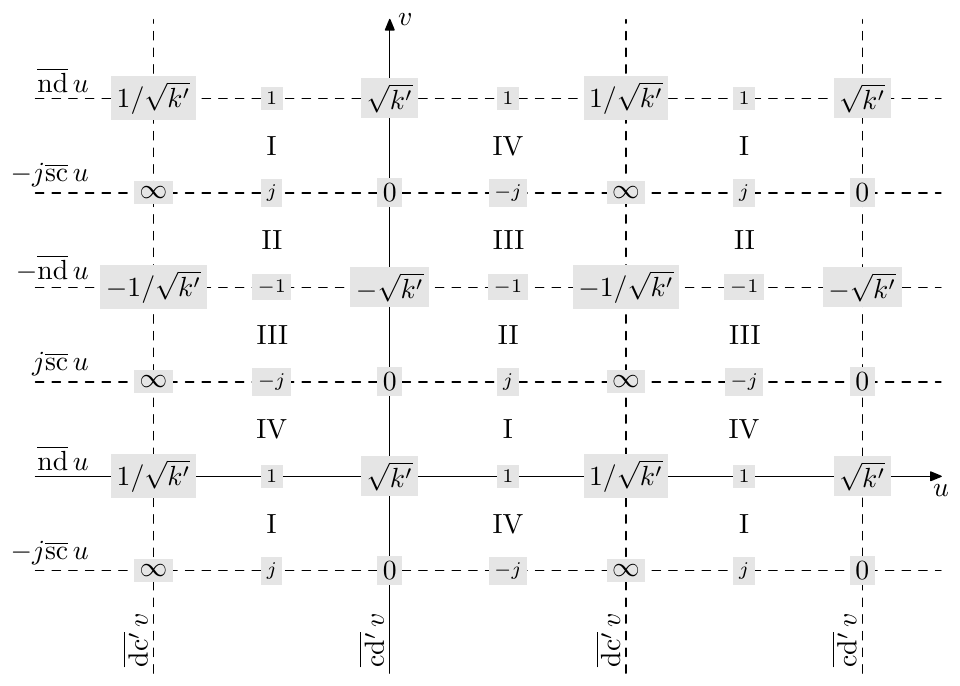
Figure 9.51: Values of on the quarter-period grid (compare to Fig. 9.44).
Derivatives
In terms of normalized functions the logarithmic derivative formulas (9.72) take the form
By checking the complex quadrants of the values of and in Figs. 9.44 and 9.45, one could establish that the first logarithmic derivative is lying in the lower complex semiplane on even imaginary periods and in the upper complex semiplane on odd imaginary periods:
or simply
where is the imaginary quarter period index.
The second logarithmic derivative is apparently lying in the upper complex semiplane if is in the I or III complex quadrant and in the lower complex semiplane if is in the II or IV complex quadrant:
or, using Fig. 9.50,
where and are respectively the real and imaginary quarter period indices.
Horizontal and vertical preimage lines of
The formulas (9.77) can be used to obtain more information about the behavior of (and respectively ) on its quarter periods. For this kind of information can be directly obtained from the complex argument formula (9.29a). For the same formula (9.71) is a bit more complicated and cannot be as easily used for analysis.
Given , we obtain:
Suppose the point is moving horizontally to the right within the -th imaginary quarter period, that is and . Then we have the following.
- By (9.80a) and (9.78)
therefore the value of is moving clockwise on even imaginary quarter periods and counterclockwise on odd imaginary quarter periods. By (9.71) and using the complex quadrants in Fig. 9.42 or 9.50 as a reference, we additionally find that
that is at integer multiples of () the value of is crossing the real and imaginary axes, starting with the real axis at . Fig. 9.52 illustrates. The family of curves generated by such horizontal preimage lines in shown in Fig. 9.53.
- By (9.80c) and (9.79)
Comparing (9.81c) to (9.81a) and (9.81b) we find that, given , the trajectories in Fig. 9.53 are speeding up when going away from the real axis and slowing down when going towards the real axis.
Now suppose the point is moving in a vertical line towards the top: , .
- By (9.80b) and taking into account (9.78)
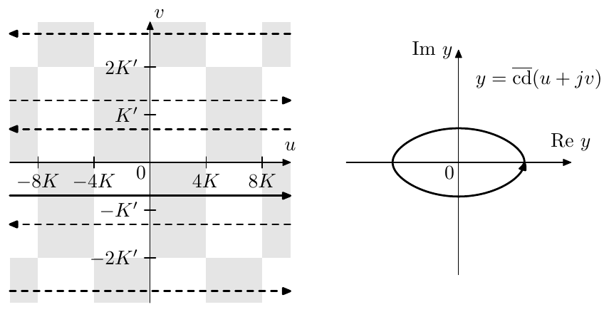
Figure 9.52: A quasielliptic trajectory and its preimages. The picture is qualitative. Particularly, the principal preimage line, shown by the solid arrow line, is actually closer to the real axis (it must be closer that ).
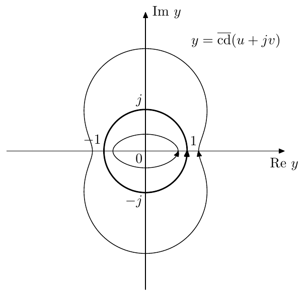
Figure 9.53: A family of quasielliptic trajectories generated from horizontal preimages . The unit circle trajectory occurs at .
where is the imaginary quarter period index corresponding to the current value of . That is will be increasing on even imaginary quarter periods and decreasing on odd imaginary quarter periods.
In fact, the movement trajectories will be as shown in Fig. 9.54, where the movement around will be occurring on even real quarter-periods and the movement around will be occurring on odd real quarter- periods. At the even boundaries the movement will be oscillating along the real line between and . At the odd boundaries the movement will be occurring along the entire imaginary axis looping through the , going downwards all the time if is even and going upwards all the time if is odd (referring to Fig. 9.50 is recommended for understanding these boundary cases). The trajectories in Fig. 9.54 complete a full cycle over one imaginary period of .
- By (9.80d) and (9.79)
Equation (9.82b) means that the second derivative of doesn’t change sign during vertical motion within a single imaginary quarter period. This doesn’t seem much, but it will be a quite useful property.
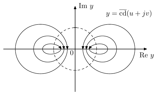
Figure 9.54: A family of trajectories generated from vertical preimages . Notice that the trajectories intersect the unit circle (shown by the dashed line) at right angles.
Since monotonic in the vertical direction on a single quarter period and is monotonic in the horizontal direction, it follows that within a single quarter-period grid cell the function is taking each value no more than once. Respectively, the quasielliptic curves in Fig. 9.53 are all distinct (that is they don’t intersect or overlap) within a single imaginary quarter-period of the domain of . Conversely, each imaginary quarter period of the domain of contains exactly one preimage of any given such curve, as shown in Fig. 9.52.
In a similar way one can argue the distinctness of the curves in Fig. 9.54.
Unit circle symmetries
In Figs. 9.53 and 9.54 we have specifically highlighted the unit circle, which is related some of the properties of . It turns out that has some symmetries in respect to the unit circle and its preimage.
Let’s take two points and , which are located symmetrically to the line on the complex plane, and consider the product
where the latest is by (9.76d). That is the corresponding values of the Jacobian elliptic cosine are conjugate-reciprocal:
and the line is the axis of the conjugate-reciprocal symmetry of . From the evenness property of the elliptic cosine (and the fact that in (9.83) is arbitrary) it follows that
that is the line is also the axis of the conjugate-reciprocal symmetry of . Since is -periodic along the imaginary axis, any other lines of the form are also the axes of the conjugate-reciprocal symmetry of :
Taking the absolute value of both sides of (9.84) we obtain
Further, assuming a purely real (so that ) the above turns into
or simply
that is the absolute magnitude of is unity on the line , exactly corresponding to the unit circle trajectory in Fig. 9.53. As another illustration, in Fig. 9.50 one could notice that is taking the values and at the intesections of vertical grid lines with the line . Since we showed that the quasielliptic trajectories in Fig. 9.53 are all distinct, there are no other points within the imaginary quarter period where , and respectively the lines are the only preimages of the unit circle.
Taking the complex argument of both parts of (9.84) we have
or
That is the complex arguments of taken at the points symmetric relatively to the line are equal.
Fig. 9.55 provides an illustration for the range . Apparently on the ends of that range the elliptic cosine has purely real values (which can be seen from the properties of and from Fig. 9.50), corresponding to the complex argument being equal to 0 or . Inside that range the value is becoming complex, where it is “maximally complex” (in the sense of having the maximal deviation from 0 or ) exactly in the middle, that is at . This corresponds to the trajectories in Fig. 9.54 crossing the unit circle at right angles, so that the tangent lines of the trajectories taken at the intersection points are going through the origin, and therefore the angular deviation from the real line is attaining a maximum at these intersection points.
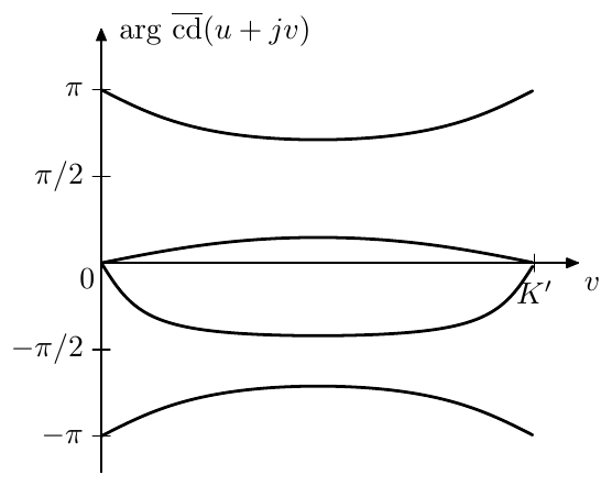
Figure 9.55: Deviation of Jacobian cosine’s value from the real axis as a function of the imaginary part of its argument, plotted for various real parts and various elliptic moduli .
In order to explain this maximum angular deviation at consider the following. The symmetry of the graphs in Fig. 9.55 is directly following from (9.86). Therefore there must be an extremum at the point in the middle of the range . By (9.82b) this is the only extremum on that range and therefore this is the point of the maximum deviation.
Since the functions , and can be obtained from by shifts and/or rotations of the complex plane (and a multiplication by or by for ), they also exhibit similar symmetries. We won’t go into detail of these. The functions and being the reciprocals of and are having similar symmetries as well.
Normalized argument
It will be also often convenient to use the following notation:
that is we write the quarter-period multiplier of the argument as a subscript of the function’s name. In this notation e.g. the real quarter-period of becomes equal to 1, therefore we will refer to this notation as normalized-argument Jacobian elliptic functions.
Note that we can’t normalize the argument simultaneously for real and imaginary quarter periods, that is we need to choose between e.g. and , depending on our needs. Noticing that
we can see that the imaginary quarter period of is and the real quarter period of is . The same obviously holds for other Jacobian elliptic functions.
Notice that Figs. 9.35 through 9.38 are effectively plotting , , and , since the argument scale is scaled by .
In Figs. 9.35 through 9.38 one could notice that the values of , , and seem to be growing (in absolute magnitude) with . Let’s see if this is always the case.
In the beginning we are going to establish the fact that the argument-normalized amplitude grows with on , that is
Before analysing the partial derivative of with respect to , we need to note the range in which is varying for :
Indeed, by (9.55) is strictly increasing for , therefore, since and , the range is mapped to and vice versa. Therefore is monotonically changing from 0 to for changing from 0 to , and respectively is monotonically changing from 0 to for changing from 0 to 1.
Now, given , by (9.57)
Since we are interested in the partial derivative of with respect to , we will consider to be fixed and and varying in the above equation. Then, taking the logarithm, we have
or
Let’s take a full derivative in respect to of both sides, where, since , the respective term fully disappears:
Since , we have and thus
Since by (9.55)
it is suffcient to show that
and then will automatically follow.
The previous inequality can be equivalently rewritten as
or, noticing that and reintroducing the explicit argument notation ,
Obviously the integral in (9.89) is positive for any and and therefore (9.87) holds. It follows that
Notice that we have allowed in (9.90). Strictly speaking, at the integral in (9.89) turns to zero, respectively . However it doesn’t matter much: since starting with arbirarily small , we have and respectively (9.90) also holds for .
Using (9.90), (9.88) and (9.58) we obtain
Using shift and symmetry properties of we can extend the above to the entire real axis (with the exception of purely integer points where has the same values independently of ):
The same property for follows from the fact that can be obtained from by a quarter-period shift, and we have
The same property for follows from (9.90), (9.88) and (9.60). The same property for follows from (9.90), (9.88) and (9.61).
Notably, the same property doesn’t hold if the argument is not normalized by the real period . Indeed, it is easily noticed that grows with both and , therefore, given , the value of will be decreasing for growing , which means that
9.11 Landen transformations
Given an elliptic modulus and the associated quarter periods and we could desire to find another elliptic modulus, such that the period ratio13 is increased or decreased by an integer factor (compared to the original ratio ). We will specifically focus on the transformation which changes the period ratio by a factor of 2. It will be particularly (but not only) useful as a means of evaluation of Jacobian elliptic functions and their inverses.
Given an elliptic modulus and the corresponding period ratio , let denote the elliptic modulus such that the corresponding period ratio is halved: . It turns out that can be found by a simple formula: . We define the ascending Landen transformation:
It is easily verified that , which explains the name “ascending”. Intuitively, an increase of the elliptic module increases the real period and reduces the imaginary period , therefore the ratio is also reduced.
Inverting the ascending Landen transformation we obtain the descending Landen transformation:
where is the corresponding complementary modulus.14 The readers are encouraged to check that . Obviously, the descending Landen transformation doubles the period ratio .
It is easily found that the ascending and descending transformations are dual with respect to swapping and (or, which is the same, and ):
where denotes the elliptic modulus complementary to . Another property which follows from (9.92) is
which also can be equivalently written as
Landen sequences of elliptic moduli
Given some elliptic modulus , Landen transformation establishes a bilateral sequence of elliptic moduli:
where . Due to (9.93) this also automatically establishes a sequence of complementary moduli
where . Note that by (9.94) we have
At small (9.92b) turns to
Thus, as grows, the moduli quickly decrease to zero. Conversely, quickly grows to 1. E.g. starting at we have a sequence
At this point the “trigonometric” elliptic functions become practically equal to their trigonometric counterparts (recall the property (9.62)), while the real quarter period becomes practically equal to . Thus we almost exactly know the value of the real quarter period and we also can evaluate the respective trigonometric functions instead of an elliptic ones. Using the relationships that we are about to establish below, one can relate the elliptic function values at to the values at larger , which then provides a way to evaluate the elliptic functions for arbitrary . Obviously, the same applies to the “hyperbolic” elliptic functions at .
Ascending recursion for quarter period
Landen transformation changes the real quarter period as
(where is the complete elliptic integral of the first kind).
Considering the sequence (9.95), let , denote the real and imaginary quarter periods corresponding to moduli . By (9.98)
One can verify that (9.99) are in agreement with the fact that the period ratio is changed by a factor of 2:
where we have used (9.99) and (9.96).
The formula (9.99a) can be used as a means to compute (for ). Notice that as is getting small, the factors are becoming very close to one. Therefore
by (9.56) should converge to . In practical computations, starting from some the factor will be indistinguishable from one within the available computation precision, and so (by (9.97)) will be the subsequent factors. At this point the computations may be stopped and we can assume that within the computation precision. Respectively
Thus we arrive at the following algorithm.
Given we wish to evaluate . Use descending Landen transformation to build a sequence of decreasing moduli , until at some step the values becomes sufficiently small so that within the available computation precision. Then ascend back to using (9.99a), thereby computing .
Using (9.100) the same algorithm can be expressed iteratively rather than recursively:
// compute K from k
K := pi/2;
for i:=1 to 5 do
    k' := sqrt(1-k^2);
    k := (k/(1+k'))^2; // descending Landen transformation
    K := K*(1+k);
endfor;
Ascending recursion15 for and
Let’s introduce the notation , etc. Note that thereby the imaginary period of is halved compared to . Let’s also introduce the notation for the arithmetic average of and its reciprocal :
Then
For the purposes of numeric evaluation it is usually more practical to rewrite (9.101a) in the form:
which particularly avoids the division by zero if .
Substituting for in (9.101) and using the shift property (9.66) we obtain
or the version for numeric evaluation:
The formulas (9.101), (9.102) can be used to compute the elliptic sine and cosine for by using a similar approach to how we used (9.99) to evaluate . Let’s start with the elliptic cosine. The idea is that by (9.62)
Now notice that in (9.102b) we have within the available computation precision, provided
within the same computation precision. Apparently, at this moment the sequence (where ) converges to .
The condition (9.103a) is the same that we had in the evaluation of . However additionally we have the requirement (9.103b) which is redundant if is real (since then ), but becomes essential if .
Since we don’t know the value of in advance, we can’t directly estimate at which (9.103b) begins to hold. Simply assuming that (9.103a) will suffice is not the best idea, since can easily have values comparable to or exceeding in absolute magnitude. Suppose however that
that is the imaginary part of the argument of doesn’t exceed half of the imaginary quarter period.16 From our previous discussion of the behavior of and we should remember that attains unit values in the middle of the imaginary quarter period and that its absolute magnitude grows away from the real axis (within the first imaginary quarter period). That is
Respectively
and
Thus we have established that under the condition (9.104) the values of do not exceed in absolute magnitude. Apparently this is by far not good enough for (9.103b) to hold, since we only guarantee that , however the situation will improve if we decrease by one or more steps.
First notice that if (9.104) holds at some , then it will hold and so will (9.105), therefore and . Under further assumption of (9.103a), from (9.102b) we have
However by (9.97) we have and therefore
That is will turn essentially to zero after just decreasing by one step and respectively the sequence (for ) will immediately converge.
In principle, we could now allow to be arbitrarily large. As we decrease step by step, the imaginary period of the function is doubling each time, thus sooner or later (9.104) will hold. However we don’t want to do unnecessarily many iterations, not only for performance reasons, but also because the precision losses will accumulate. Therefore it might be more straightforward to simply wrap the argument of using the imaginary periodicity property.
Thus we arrive at the following algorithm. Suppose we want to evaluate . If , we should use the periodicity property to get into the range . Then introduce and , so that we have . Then we use the descending Landen transformation to decrease to almost zero,17 where
At this point we compute instead of and ascend back using (9.102b). In pseudocode this could be expressed as:
// compute cd(x/K,k), assuming |Im x|<=K'
function cdK(u,k,steps=5)
    if steps=0 then return cos(pi/2*u) endif;
    k' := sqrt(1-k^2);
    k := (k/(1+k'))^2; // descending Landen transformation
    y := cdK(u,k,steps-1);
    return ((1+k)*y)/(1+k*y^2);
endfunction;
Notice that may be complex in the above, where we would need a cosine routine supporting a complex argument, which, if missing, could be implemented by (9.29a).
Evaluation of is done in the same way, except that we have to compute as the approximation of . The evaluation routines for sn and cd can be also reused for evaluation of sc and nd using (9.63).
Descending recursion for sn x and cd x
We could invert the formulas (9.101) and (9.102) to express and in terms of respectively or :
or its “numerical” version, avoiding the divisions by zero for
and
The ambiguity in formulas (9.106) and (9.107)18 is apparently due to the fact that the imaginary periods of and are doubled compared to and , therefore the formulas “do not know which of the two imaginary half-periods to choose”.
The descending recursion can be used to evaluate the inverses of sn and cd. Given an equation of the form (where we want to find ), we introduce , and , so that . Then we use (9.107) to descend to , where we have
with high precision and therefore we can simply find by , thereby obtaining .
Note that, even though (9.107) gives ambiguous results, any of those results will give a correct answer in the sense that we will get one of the possible solutions of at the end of the recursion procedure. However, in order to avoid getting too far away from the origin (and in order to keep within the real numbers range if is a real number not exceeding 1 in magnitude), it is recommended to choose the value with the smaller absolute magnitude from the two values of in (9.107a), or, equivalently choose the “+” sign in the denominator of (9.107b). In case of complex values “choosing the + sign” also means that the complex square root operation should yield a value with a nonnegative real part, that is we should use the principal value (9.30).
Computing the inverse of sn is done in the same way using (9.106) (where it is preferable to choose the smaller-magnitude one from the two values of in (9.106a) and to use the “+” sign in the denominator of (9.106b)), finally computing by , thereby obtaining . The respective pseudocode routine could be e.g.:
// compute x=sn^-1(y,k)
Kbypi2:=1; // accumulate ratio K/(pi/2)
for i:=1 to 5 do
    k' := sqrt(1-k^2);
    k_1 := (k/(1+k'))^2; // descending Landen transformation
    y := 2/(1+k_1) * y/(1+sqrt(1-k^2*y^2));
    k := k_1; Kbypi2 := Kbypi2*(1+k);
endfor;
x := Kbypi2*arcsin(y);
The routine for is identical, except that it should use arccos instead of arcsin. Alternatively notice that and are related via shift and symmetry properties of cd and sn,, e.g. , so that one function can be expressed in terms of the other. The functions and can be expressed via and using (9.63).
If the argument of and is restricted to real values, all respective computations will be real. Otherwise we need sqrt, arcsin and arccos functions to support complex argument, where sqrt must return the principal value (with nonnegative real part). These functions, if missing, can be implemented using (9.30) and (9.32).
We mentioned that the ambiguity of (9.106) and (9.107) is due to the doubling of the imaginary period of and on each step. Instead of that, we could have had the imaginary period fixed and the real period halved on each step, resulting in the same change of the period ratio. E.g. for the elliptic cosine, introducing , we have another relationship:
(where ).
Unfortunately, while (9.108) avoids the ambiguity of (9.106) and (9.107), it is not useful for evaluation of the inverses of sn and cd, as there is another ambiguity popping up. Due to periodicity and symmetries of along the real axis, we won’t know which of the possible values of the inverse of to take. When using (9.106) and (9.107) the real period of and was always exactly preserved by the transformation, therefore this ambiguity didn’t matter as any of the values of and would do. If however the real period is not kept intact, the value returned by might result in a wrong value after rescaling back to the original periods and .
One further issue is related to the preservation of the imaginary period. Particularly the range is mapped to the range , respectively for a real above that range (that is ) we obtain a real . Respectively will return a purely imaginary result (while what we expect from is clearly not purely imaginary, as one can see e.g. from Fig. 9.42) no matter how many times we apply the recursion (9.108) before evaluating the inverse cosine.
Ascending recursion for nd x
Using the imaginary argument property (9.63) of the elliptic cosine and the Landen transformation’s duality (9.93) we can convert the descending recursion formula (9.108) for cd into an ascending recursion for , which takes the form
The main value of this recursion formula for us will be that we’ll use it to derive another transformation.
Double Landen transformation
Consider two subsequent Landen transformation steps occurring from to . Inverting (9.108) we obtain
Now we switch to the real period-based notation by substituting . This is also equivalent to since and thus . Therefore the substitution replaces with and with , resulting in
Inverting (9.109) we obtain
By (9.69)
Solving for :
By (9.92) and (9.93)
where we have noticed that the obtained expression can be conveniently written in terms of the Riemann sphere rotation . Therefore
Continuing the transformation of we obtain
and thus
or
where the respective elliptic modulus is found from (9.110).
Notice that the halving of the argument in (9.111) is matched by the fact that the period ratio is changed by a factor of 4, That is . At the same time the real and imaginary periods of are 4 and , while the real and imaginary periods of are 4 and . Thus we have identically periodic functions in the left- and right-hand sides of (9.111).
9.12 Elliptic rational functions
Landen transformation was changing the period ratio by a factor of 2, which resulted in various elliptic functions after the transformation being expressed as a rational function of the same elliptic function prior to the transformation. There is a generalization of Landen transformation where the period ratio is changed by an arbitrary positive integer factor . Such transformation is referred to as N-th degree transformation and the factor is referred to as the degree of the transformation.
Suppose we are having an elliptic modulus with respective quarter periods and . Let be another elliptic modulus with respective quarter periods and , such that the quarter period ratio is increased times:
(the equation (9.112) is referred to as degree equation). Notice that since the period ratio is increased, the modulus is decreased: .
Apparently and are interdependent, where from (9.112) we obtain that increasing decreases the ratios and , and thus increases as well. Thus is an increasing function, where at equal to a power of 2 we obtain a times repeated Landen transformation. The way to compute from a given (and back) for arbitrary will be discussed later.
In the transformation from to we wish to obtain the relationship for cd, such that the imaginary period (in terms of normalized argument) is fixed. It turns out that such relationship always has the form:
where , and is some real rational function of order . We already had a particular case of this formula for in (9.108) where
The function is referred to as elliptic rational function of order N. Notice that depends on the elliptic modulus , even though we don’t explicitly notate it as function’s parameter. Example graphs of are given in Fig. 9.56.
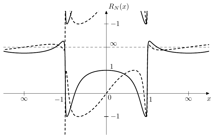
Figure 9.56: Elliptic rational functions of even (solid) and odd (dashed) orders for . The graphs do not cross the horizontal axis at , rather , however the resolution of the figure is insufficient to see that. The poles of are occurring at the intersections of the respective graph with the thin horizontal dashed line at .
By using (9.112) we could rewrite (9.113) in terms of the real periods:
where , . We could also rewrite (9.113) and (9.115) in a form without argument normalization, giving:
Notice that any of the formulas (9.113), (9.115), (9.116) implies that
(with the properly chosen elliptic moduli for each of , and ), as we are effectively simply chaining an N-th and an M-th degree transformation.
as representation of linear scaling
In an obvious way, equation (9.113) can be expressed in terms of the preimage domain:
Alternatively, (9.115) can be expressed as
Differently from , and , this time there are two different mappings from the preimage to the representation domain in each case, corresponding to the two different moduli and . The linear scaling is explicitly present only in (9.119), however this is purely due to the implicit scaling contained in the period-normalized notation. The explicit notation form is the same for both (9.118) and (9.119) and contains the linear scaling:
The mappings are however still different, since .
By (9.112) the scaling (9.120b) exactly matches the imaginary periods and expands a single real period to exactly real periods. For that reason the shifts of by an integer number of real and/or imaginary periods do not affect the values of and . By the even symmetry of cd a change of sign of doesn’t affect the values of and either. This however exhausts the set of possible preimages of a given , since, as we know, takes each value only once per quarter-period grid cell (where the complex quadrants in Fig. 9.42 provide additional reference). Thus we can pick any preimage of as the value of and therefore can rewrite (9.118), (9.119) and (9.120) in their respective explicit forms:
where denote the inverse functions of the respective cd functions. Equation (9.121c) is the commonly known explicit expression for elliptic rational functions.
As with and , an important class of preimages will be the horizontal lines in the complex planes and . From our discussion of cd and we should recall that these lines produce distinct quasielliptic curves as their respective images, the full cycle of these curves corresponding to a single real period of or respectively (Figs. 9.52 and 9.53 serve as reference). Therefore moving in such quasielliptic curve will be mapped to moving in a similar curve, each cycle of producing cycles of .
Recall that with cosine-based preimages we were preferring the preimages in the lower complex semiplane, so that preimage movement towards the right was corresponding to counterclockwise rotation in the representation domain. Similarly, we are going to choose the elliptic cosine-based preimages within the imaginary quarter period strip located immediately below the real axis, as shown in Fig. 9.52, therefore preimage movement towards the right will correspond to counterclockwise rotation in the representation domain.
Given a preimage located in the imaginary quarter period immediately below the real axis, the preimage will also be located in the imaginary quarter period immediately below the real axis, since the imaginary quarter periods of are mapped exactly onto the respective imaginary quarter periods of . Also, apparently, and either both move simultaneously to the right or both to the left. Thus and move either both counterclockwise or both clockwise.19
Bands of
The four different parts of the principal preimage of the real line in Fig. 9.47 will correspond to the bands of elliptic filters which we are going to construct later. It is convenient to introduce the respective terminology at this point already.
In terms of (9.120) the principal preimage of the real axis is
Respectively the principal preimage of the real axis is:
The linear scaling (9.120b) maps (b) to one-to-one (imaginary period is preserved). The mapping from (a) to and from (c) to is one-to-N (real period is multiplied by ). This is responsible for the appearance of the equiripples for and in Fig. 9.56. The mapping from (c) results either in some (non necessarily principal) preimage if is odd or in a non-principal preimage if is even.
Naming these four bands of after the respective bands of the elliptic filters, we have:
| Passband | ||
| Two transition bands | ||
| Stopband |
The readers are advised to compare the above results to Fig. 9.56, identifying the equiripples of amplitudes and in the pass- and stop-bands respectively. Since is very close to 1, the transition bands are very narrow and aren’t visible in Fig. 9.56, however at smaller the stopband equiripples would become too small to be visible in the same figure.
The value is determining the width of the transition band(s) and is therefore referred to as the selectivity factor. The value determines the ratio of the equiripple amplitudes in the pass- and stop-bands and is referred to as the discrimination factor. Since and increase or decrease simultaneously, so do and . Therefore decreasing the transition band width (which is the same as decreasing the selectivity factor ) decreases the discrimination factor of , thereby making the stop-band equiripples larger. Thus there is a tradeoff between the transition band width (which we, generally speaking, want to be small) and the discrimination factor (which we, generally speaking, want to be large). Fig. 9.57 illustrates.
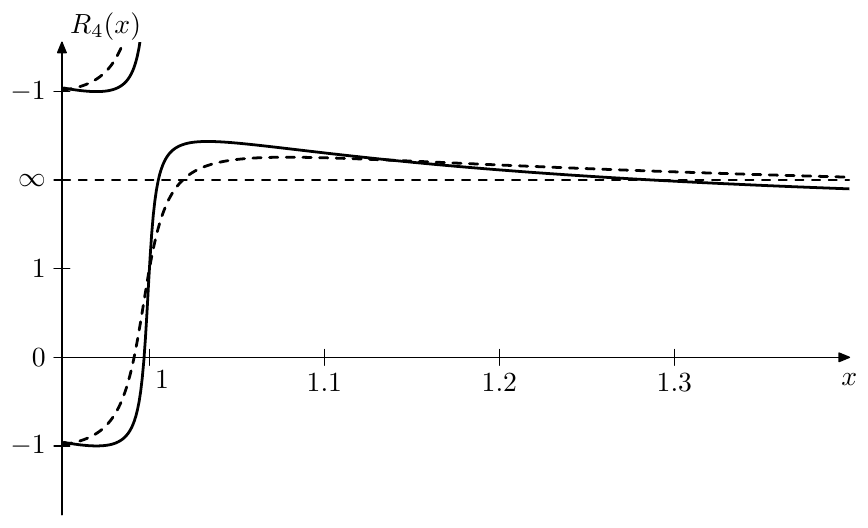
Figure 9.57: Transition region of for (solid) and (dashed). The horizontal axis is linear, the vertical axis is using the arctangent scale.
Even/odd property
Since , a negation of corresponds to a shift of its preimage by . Respectively is shifted by , which will result in a negation of if is odd and will not change is is even. Therefore is even/odd if is even/odd:
Values at special points
The principal preimage of is . Therefore and . Therefore
By (9.122)
The principal preimage of is . By (9.112) and . Therefore
By (9.122)
Since equiripples begin exactly at the boundaries of the respective bands of , the values at and also give the amplitudes of the equiripples of , which are thereby 1 in the passband and in the stopband.
The principal preimage of is . By (9.112) and
The principal preimage of is . By (9.112) . With the help of (9.65) we reuse the result for , obtaining
Two other interesting points are logarithmic midpoints of the transition band occurring at . The princial preimage of is the transition band’s preimage midpoint and respectively . Thus
That is the logarithmic midpoint of the transition band is mapped to the logarithmic midpoint of the respective value range . By (9.122)
Normalized elliptic rational functions
The graphs of in Fig. 9.56 look somewhat asymmetric regarding the boundaries of the bands, which are at and and the amplitudes of the ripples which are and respectively. This can be addressed by switching to normalized elliptic cosine. The equations (9.113), (9.115) and (9.116) thereby respectively turn into
while (9.120) turn into
and (9.121) turn into
where
is the normalized elliptic rational function. Note that is essentially simply a notational shortcut for the right-hand side of (9.126), however due to the more pure symmetries, it is often more convenient to work in terms of than .
The bands of are therefore
while the special points of respectively are:
The graphs of are plotted in Fig. 9.58.
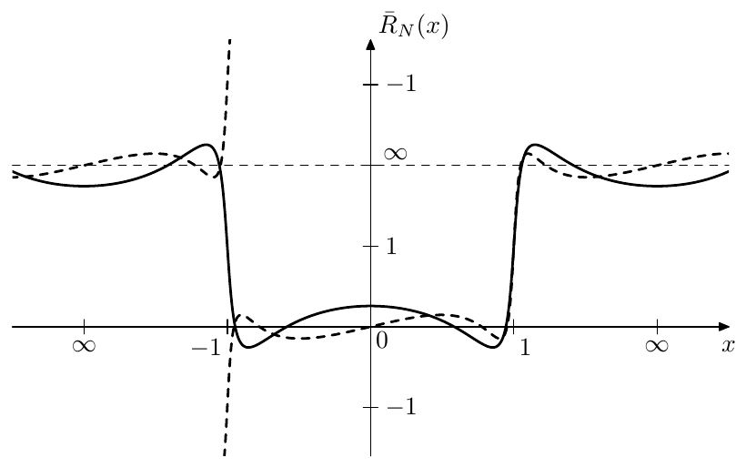
Figure 9.58: Normalized elliptic rational functions of even (solid) and odd (dashed) orders for .
The interpretation of as a linear scaling representation is essentially the same as in (9.118), (9.119) and (9.120) respectively, except that cd must be replaced with . E.g. (9.120) becomes
Notice that the chain rule (9.117) works in the same form for normalized elliptic rational functions:
since the elliptic modulus for one stage is equal to the elliptic modulus for the next stage, thus the coefficients and cancel between each pair of stages.
Symmetries of
In Fig. 9.58 one can notice that the graphs of have certain symmetries. One symmetry is relatively to the origin:
(which is simultaneously the symmetry relative to ). Apparently this is simply the even/odd property of which is preserved in the form.
The other symmetry is relatively to the point :
with a similar symmetry around the point at which follows from the first two symmetries. The proof of (9.130) follows from (9.75d). Given and its preimage , the preimage of is . Similarly, the preimage of is , however simultaneously
therefore is also the preimage of and .
In terms of the symmetry (9.130) takes the form
Similarly to , the normalized elliptic rational function maps the quasielliptic curves Fig. 9.53 to other quasielliptic curves from the same family. By Fig. 9.53 and (9.85) the unit circle will be mapped to the unit circle, since the preimage line will be mapped to the preimage line . There won’t be other preimages of the unit circle, since all trajectories in Fig. 9.53 are distinct and occur for different imaginary parts of the preimage. Thus
Poles and zeros of
Letting and using the representation form (9.119) we obtain
(where the second form is given for comparison with the respective derivations of the zeros of and ). Respectively
and
which means that the zeros of are
where there are distinct values corresponding to . Notice that the zeros are all real and lie within . Also notice that , therefore the zeros are positioned symmetrically around the origin. Consequently, if is odd, one of will be at the origin.
By (9.131) the poles can be obtained from zeros as
Note that if is odd, then so is and one of the zeros will be at . In this case one of the poles will be at the infinity and there will be only finite poles.
Given and taking into account that , we can write in the form
which we could also write as
The value of the gain coefficient can be obtained from the fact that must satisfy . Alternatively we can satisfy by simply forcing each of the factors of to be equal to unity at (where prior to the factor normalization we also have multiplied each of the factors by )
Poles and zeros of
By (9.126) the zeros of can be obtained from the zeros of as
Notice that thereby . By (9.130) the poles are related to the zeros as
The factored form (9.134) respectively becomes
where we don’t have explicit normalization factors anymore, since the factors under the product sign are already all equal to unity at , thereby giving as the transition band’s midpoint (which is exactly what it should be according to the previously discussed special point values of ).
By obtaining equations (9.134) and (9.136) we have constructed and in the explicit rational function form.
Relationship between and
Note that the explicit rational function forms (9.134) and (9.136) were obtained without using the yet unknown to us (or or ). On the other hand, having constructed and/or , we can obtain from the condition or .
We can also obtain an explicit expression for in terms of . Substituting (9.134) into we obtain
By (9.133) where
Therefore
where the latter transformation is by (9.68). Noticing that
we obtain
(where the number of factors under the product sign is equal to the integer part of ) which formally gives an explicit expression for . However practically this expression is exactly the same as and thus we can simply find (and respectively ) from the latter condition.
Finding from can be done by using the duality of the -th degree transformation in respect to and (which is pretty much the same as the respective duality of the Landen transformation). Let denote the -th degree transformation of defined by (9.137) (or by explicit usage of or ). If the ratio is decreased times by the -th degree transformation from to , then the ratio is increased times, which means we are performing an -th degree transformation from to , that is . Conversely, and are related via an -th degree transformation: , which by (9.137) means
Renormalized elliptic rational functions
Similarly to renormalized Chebyshev polynomials we introduce renormalized elliptic rational functions where we will renormalize only (although we could take similar steps to renormalize as well):
As with renormalized Chebyshev polynomials, the parameter affects the bands of the elliptic rational functions and the equiripple amplitudes. Apparently the passband of is , while the stopband is . Thus if becomes smaller, the passband shrinks while the stopband simultaneously expands and vice versa. The equiripple amplitudes in the pass and stop-bands are becoming equal to and respectively. Therefore both values increase if grows and decrease if becomes smaller, which means that the equiripple sizes in the pass- and stop-bands are traded against each other20 (Fig. 9.59). Notice that thereby a smaller bandiwth of the pass- or stop-band corresponds to a smaller equiripple amplitude in the same band and vice versa.
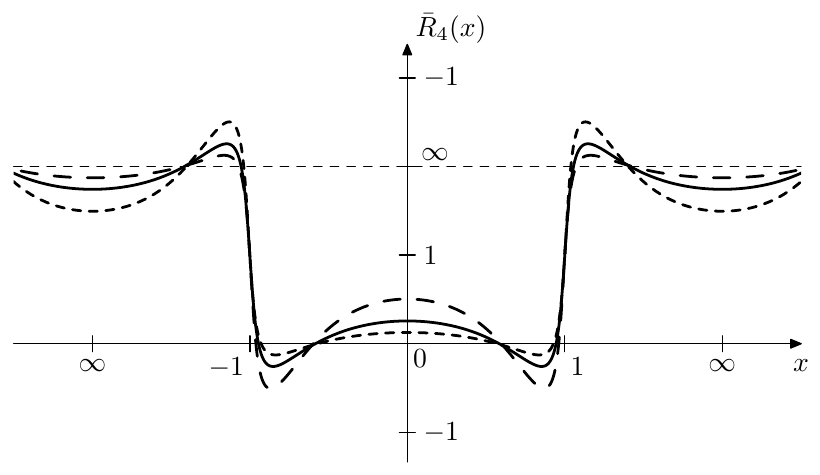
Figure 9.59: Renormalized elliptic rational function for (solid), (small dashes) and (large dashes). As the used elliptic modulus is pretty close to , the corresponding variations of the transition band width are not well visible.
The reasonable range of is equal to the transition band . For within this range the equiripples (both in the pass- and stopbands) do not grow further than to unit amplitude. As a somewhat excessive range of we could take , limiting between the zeros and poles of . In this case the equiripples may become arbitrarily large.
As with renormalized Chebyshev polynomials, we may omit the parameter , understanding it implicitly, and simply write .
Relation to , and
In (9.136) it is easily noticed that at the right-hand side turns into . On the other hand , therefore, if , then and respectively by (9.136)
or simply for (Fig. 9.60).
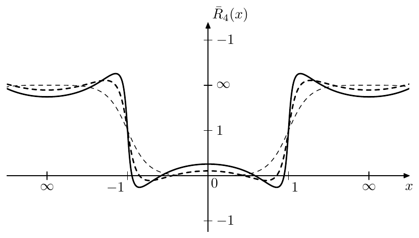
Figure 9.60: Normalized elliptic rational function for (solid), (dashed) and (thin dashed).
At we have and , therefore (9.115) turns into
By replacing with it can be equivalently written as
which is identical to (9.35). Therefore becomes identical to and thus we have
or simply for . Notice that as and , the transition band of becomes infinitely large in both preimage and representation domains, while the stopband disappears into infinity.
Using (9.126) and (9.139) we can express the approaching to in terms of and :
where we had to take the limit to avoid divisions and multiplications by zero. By the definition of equation (9.142) can be rewritten as
Substituting for and reciprocating both sides
By (9.130) and (9.139)
Transition band slope of
By (9.140) turns into at . On the other hand at the transition band’s midpoint we have . It would be therefore interesting to compare the slopes of and within the transition band. In order to do that we are going to take similar steps to what we did in the comparison of and . Comparing (9.136) to (9.40) we compare their individual factors by computing their respective differences:
Assuming , we have in the above. Thus in the range the differences (9.144) are strictly positive and the factors of (9.136) are larger than those of (9.40). Since for all factors of (9.136) and (9.40) are positive, we have
By the even/odd symmetries of and :
By the symmetry (9.130) and by the same symmetry of
Note that thereby our discussion has completely covered the band which also includes the entire transition band . From (9.144) we can also notice that the difference grows in magnitude as grow in magnitude. However by (9.135) and (9.91) the absolute magnitudes of should simply grow with . Thus the differences (9.144) grow with and respectively deviates stronger for within the transition band as grows (which can be seen in Fig. 9.59).
In order to explicitly compute the derivative of at the transition midpoint , we will evaluate the derivative of at (which is the point where ). By (9.72)
We already know that . The value of can be obtained by (9.69) giving
By Fig. 9.44, (9.63) and Fig. 9.36 we choose the positive result of taking the square root
By (9.66)
Thus
Now by (9.127) the function is obtained as a sequence of three transformations. Differentiating each of these transformations at the point corresponding to we obtain
and thus
At we have , and therefore corresponding to the fact that . At higher the derivative grows (Fig. 9.61).
In order to convince ourselves that for we could notice that , and , therefore . Now, for a given , the value will obviously decrease with growing (as we are using a higher degree transformation of the period ratio). Therefore can be bounded from below by its own value at . A bit later in the text we will obtain an explicit expression for where it will be obvious that as . Therefore at , and so it does for all other .
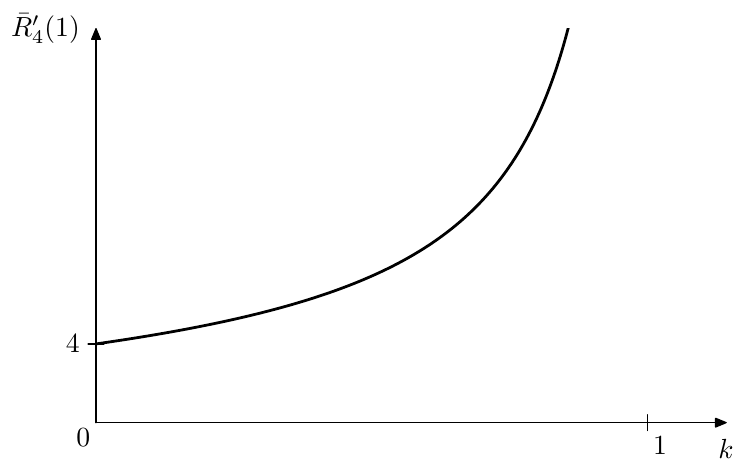
Figure 9.61: Transition midslope derivative of for various .
Transition band slope of
By (9.141) the elliptic rational function turns into a Chebyshev polynomial of the same order . We would be now in the position to compare their slopes within the transition band of .
Comparing the factors of (9.134) and (9.42) (where in (9.42) we let to turn into ) we first pretend that the zeros of and are identical. In that case the difference of the respective factors is
Since within the transition band of we have and , the difference (9.146) is positive for (for ).21
By (9.133) and (9.91) the zeros grow with . On the other hand, the zeros of become equal to Chebyshev polynomial’s zeros at . Thus the zeros of are smaller in absolute magnitude than those of . Temporarily notating Chebyshev polynomial’s zeros as where (assuming ), we notice that
where we have used (9.43). That is the difference (9.147) is again positive for and it is growing with (which corresponds to the growing ). Adding (9.147) and (9.146) we obtain
where . By our preceding discussion (9.148) becomes larger at larger .
Since all involved factors are greater than unity in the transition band of , it follows that in that range and the difference grows with . By even/odd symmetries of the respective functions we have
and the difference becomes larger with .
Elliptic rational functions of order
Constructing an elliptic rational function of a power-of-2 order is especially easy, since we can combine the explicit expression (9.114) for with the chain rule (9.117) to build functions of other power-of-2 orders.
It is therefore also helpful to have a ready explicit expression for . By (9.114) and (9.126)
Recalling that for
we further obtain
Multiple expressions of the form (9.149) (with different related through Landen transformation) can be chained to obtain for other power-of-2 orders.
The derivative at is
It is left as an excercise for the reader to verify that (9.150) is a particular case of (9.145).
Notably, by (9.110), the formula (9.150) can be rewritten as where is a complementary modulus to where .
9.13 Elliptic filters
Elliptic filters are obtained by using renormalized elliptic rational functions as in (9.18).22 The main motivation to use renormalized elliptic rational functions instead of and is that, as we already know they grow faster than and within their transition bands, which results in a steeper transition band’s slope. The tradeoff is that in order to achieve a steeper transition band we need to allow ripples in the pass- and stop-bands.
Thus, in (9.18) we let
that is
The parameter of is affecting the equiripple amplitudes of and thereby the equiripple amplitude in the pass- and stop-bands of . It is convenient to introduce the additional variable
Using (9.151) we particularly may write
Given a desired filter order , we still have two further freedom degrees to play with, corresponding to the parameters and , where, as we should recall from the discussion of elliptic rational functions, defines the tradeoff between the transition bandwidth and the ripple amplitudes, and defines the tradeoff between the ripple amplitudes in the pass- and stop-bands. One of the possible scenarios to compute the elliptic filter parameters can be therefore the following. Suppose we are given the desired filter order and the desired pass- and stop-band boundaries (where the passband boundary must be to the left of and the stopband boundary must be to the right of ). Recalling that the pass- and stop-bands of are (in the positive frequency range) and respectively, we can find and .
Another scenario occurs if we are given the discrimination factor . By (9.137) this defines selectivity factor and respectively the transition band width, but we can still play with to control the tradeoff between the pass- and stop-band ripples.
Since the passband amplitude of is , the amplitude response is varying within in the passband. Since the stopband amplitude of is , the amplitude response is varying within in the stopband. The value of therefore affects the tradeoff between the equiripple amplitudes of in the pass- and stop-bands. Since depends on , this is consistent with our previous conclusion that affects the tradeoff between the equiripple amplitudes of , where a smaller bandwidth of the pass- or stop-band corresponds to smaller equiripples within the respective band. Remember that the range of is generally restricted to (or just a little bit wider). Fig. 9.62 illustrates.
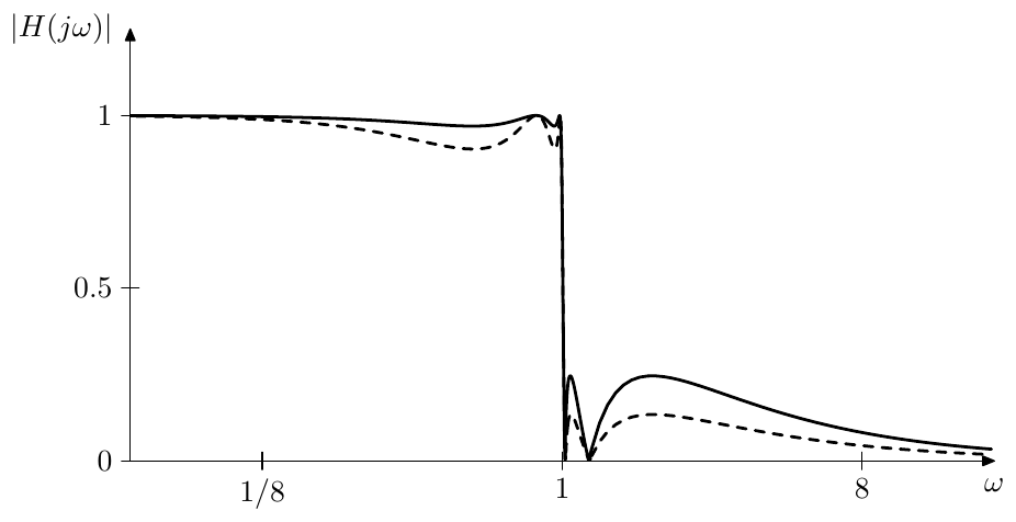
Figure 9.62: Elliptic filter’s amplitude responses for , and (solid) and (dashed). Notice the usage of the linear amplitude scale, which is chosen in order to be able to show the amplitude response zeros.
Poles of elliptic filters
Since is a rational function, the transfer function defined by (9.18) will have poles and zeros. The equation for the poles of is
or
or
or, introducing
where the “+” sign corresponds to the even poles and the “-” sign to odd poles.
Recall the interpretation of as a representation of linear scaling of the preimage, which is given by (9.127). Suppose is moving in a counterclockwise direction in a quasielliptic curve which is a representation of some preimage line (Figs. 9.52, 9.53). Earlier we have agreed to chose the preimages within the imaginary quarter period right below the real axis, that is . In this case the counterclockwise movement in the representation domain assumes that is moving towards the right.
Since , the corresponding line in the preimage of is , where . Therefore , that is the line also goes within the imaginary quarter period right below the real axis. Obviously, since moves towards the right, so does , and moves in a counterclockwise direction.
We wish to pass through the points going counterclockwise. By (9.71) the intersections of the quasielliptic curve with the imaginary axis are occuring at , therefore we choose
(which thereby belongs to )23 and
According to (9.71) the purely imaginary values of are attained when the real part of the elliptic cosine’s argument is equal to , where . Thus, the values will be attained by at
where, since , the value is attained at and other even values of . Thus, the solutions of the even pole equation will occur at even values of . Fig. 9.63 illustrates.
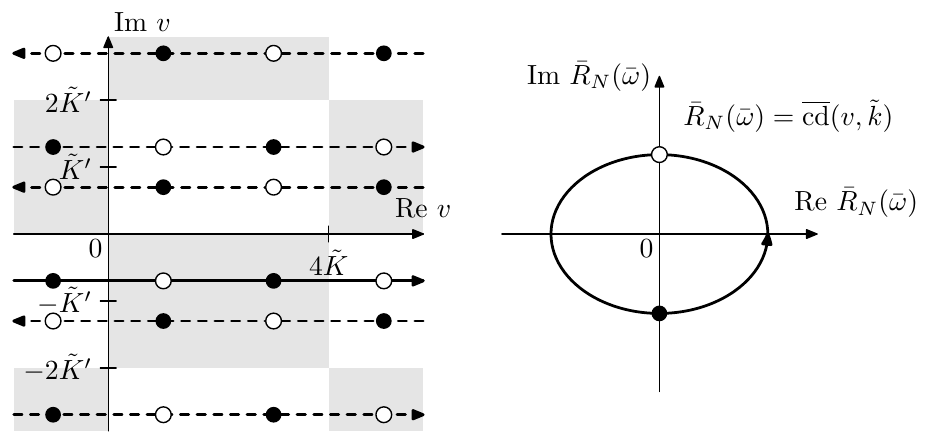
Figure 9.63: Preimages of (qualitatively).
From (9.154) we obtain
where there are essentially different preimages of occuring at consecutive values of all lying on the line . Going back to the representation domain we obtain lying on the respective quasiellipse:
Fig. 9.64 illustrates.
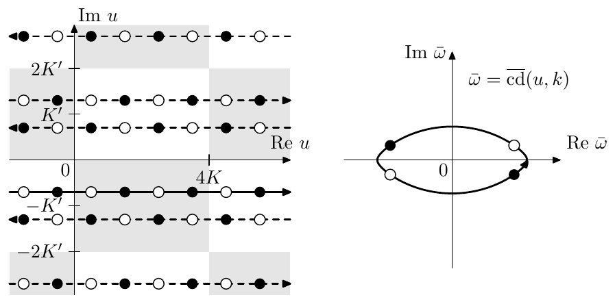
Figure 9.64: Transformation of Fig. 9.63 by (for ). The white and black dots on the quasielliptic curve are even/odd elliptic poles in terms of . (The picture is qualitative.)
Switching to :
It is easily checked that the values of are moving counterclockwise starting from the positive real semiaxis, where the values occurring at even/odd correspond to even/odd poles respectively.
Switching from to we obtain the expression for the poles:
Since the values of are moving counterclockwise starting from the real positive semiaxis, the values of are moving counterclockwise starting from the imaginary “positive” semiaxis, which means that starting at we first obtain the stable poles at . The next values of will give the unstable poles.
For filter orders which are powers of 2 one can solve the equation (9.153) in an easier way using (9.149) and (9.128).
Zeros of elliptic filters
The zeros of , if expressed in terms of coincide with the poles of , which can be found from the poles of as , where are given by (9.135). By the zeros can be reexpressed in terms of . For filter orders which are powers of 2 there is a simpler way using (9.149) and (9.128).
One should remember that for odd the function has a zero at the origin which doesn’t have a corresponding finite pole of , respectively there is no corresponding finite zero of and no corresponding factor in the numerator of . Respectively the order of the numerator of is rather than , and the zero at the inifinity occurs automatically due to the order of the numerator being less than the order of the denominator. Fig. 9.65 provides an example.
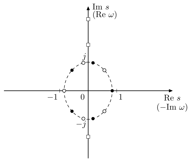
Figure 9.65: Poles (white and black dots) and zeros (white squares) of an elliptic filter of order . Each of the zeros is duplicated, but the duplicates are dropped together with the unstable poles.
In Fig. 9.65 one can notice that the poles are more condensed closer to the imaginary axis. Apparently, this is due to (9.81c) and the related explanation.
Gain adjustments
The default normalization of the elliptic filter’s gain is according to (9.18):
which thereby defines the leading gain coefficient of the cascade form implementation (8.1). We could also find the leading gain from the requirement , but we should mind the possibility of accidentally obtaining a phase response at .
With the leading gain defined this way the amplitude response varies within in the passband. We could choose some other normalizations, though. E.g. we could require . Or we could require the passband ripples to be symmetric relatively to the zero decibel level, which is achieved by multiplying (9.156) by :
so that varies within within the passband.
Elliptic minimum Q filters
At we have , thus attains the reciprocal symmetry (9.130). Simultaneously, by (9.151) , respectively
while (9.155) turns into
By Fig. 9.53 and (9.85) the poles of are all lying on the unit circle.24 Further, by Figs. 9.54, 9.55 and the associated discussion, the values of in (9.157) are having the maximum possible angular deviation (among the ones arising from different values for ) from the real axis. Respectively, the poles given by (9.157) are having the maximum possible angular deviation from the imaginary axis, which means that the corresponding cascade 2-pole sections will have the minimum possible resonances. Therefore elliptic filters arising at are referred to as elliptic minimum Q filters, or shortly EMQF.
Butterworth and Chebyshev limits
By (9.140) at EMQF filters turn into Butterworth filters. By (9.142) at and elliptic filters turn into Chebyshev type I filters. By (9.143) at and elliptic filters turn into Chebyshev type II filters.
Summary
Classical signal processing filters are defined in terms of the squared amplitude response equation (9.18). By choosing different function types as in (9.18) one obtains the respective filter types:
| Filter type | Definition |
|---|---|
| Butterworth | |
| Chebyshev type I | |
| Chebyshev type II | |
| Elliptic |
-
The general discussion of the idea of the Riemann sphere is not a part of this book. Readers unfamiliar with this concept are advised to consult the respective literature. ↩
-
One could also notice that (9.10) are very similar to the bilinear transform and its inverse, where the latter two have an additional scaling by . ↩
-
This is also the reason for the notation : the subscript simply indicates the result of the transformation of . ↩
-
We specifically leave it undefined, whether or for negative real numbers, as this is anyway a line on which the principal value of has a discontinuity and thus, considering the usual computation precision losses, one often can’t rely on the exact value of being returned for . ↩
-
Notice that the principal preimage in Fig. 9.16 doesn’t necessarily coincide with the set of values returned by the formulas (9.32), particularly since the arccos formulas in (9.32) exhibit discontinuities either for or for real . The main reason to choose this specific preimage is that its generalization to the case of Jacobian elliptic cosine will be convenient for our purposes. ↩
-
Classically, Chebyshev filters are obtained from Chebyshev polynomials by letting where is some small value. This way however usually requires some cutoff correction afterwards. The way how we introduce Chebyshev filters is essentially the same, but directly results in a better cutoff positioning. One way is related to the other via (9.44) combined with a cutoff adjustment by the factor . ↩
-
This choice is arbitrary, we simply better like the option of increasing real part of . Alternatively we could let the real part of decrease, obtaining . However then we would need to have a negative coefficient in front of in (9.46). ↩
-
It might seem that the imaginary semiaxes of the ellipses in Figs. 9.26 and 9.27 are of unit length. This is not exactly so, although they are very close, being equal to approximately 1.00003 and 1.00004 respectively. ↩
-
Alternatively one could notice that the poles of Chebyshev type II (lowpass) filters are identical to the poles of Chebyshev type I hipass filters, since both can be obtained from the poles of Chebyshev type I lowpass filters by the LP to HP transformation. If Chebyshev type II lowpass poles are obtained this way, the order of their enumeration will be symmetrically flipped relatively to the one of the prototype Chebyshev type I lowpass poles. That is, if Chebyshev type I poles are going counterclockwise starting from the “positive” imaginary axis, then Chebyshhev type II poles obtained by the LP to HP tranformation will be going clockwise from the “negative” imaginary axis (thereby stable poles will be converted to stable poles, but the even/odd property of the poles will be switched if N is even). ↩
-
There is yet another Jacobian elliptic function, which is simply equal to rather than . Depending on the purpose either of these functions may be referred to as elliptic cosine. Each of these two functions inherits different properties of . For the purposes of this book we will need the one defined by (9.59) and this is the one to which we will refer to as elliptic cosine. ↩
-
Both and are even functions. Therefore it doesn’t matter in which direction to rotate by . ↩
-
Note that here (and further where we specifically refer to function’s period, or half- or quarter-period) we mean the period of the function itself, rather than one of the least common periods and of all Jacobian elliptic functions. ↩
-
The ratio of the periods is of course formally speaking not but . However, obviously these values are equal. ↩
-
The second expression in (9.92b), in comparison to the first one, reduces the computation precision losses at small . ↩
-
This technique is commonly referred to as descending Landen transformation, since it expresses elliptic functions with higher values of the modulus via elliptic functions with lower values of the modulus. However the recursion formula itself is applied to compute elliptic functions with higher from elliptic functions with lower , thus the recursion itself is ascending. ↩
-
Notice that we needed to divide by in (9.104) because the notation includes the automatic multiplication of the argument by . ↩
-
Note that thereby after one iteration we are guarateed that . ↩
-
Note that the inverse of gives two different values. ↩
-
Obviously, we could have chosen any other imaginary quarter period preimage strip. We have chosen the one right below the real axis simply to have a better defined reference in the preimage domain. ↩
-
By the earlier given definition of the amplitude of oscillations around infinity, the size of the stop-band equiripples is smaller if the formal amplitude of the equiripples is larger. ↩
-
Actually the same holds a bit further than within the tranistion band, namely within but for simplicity we’ll talk of transition band. ↩
-
Classically, elliptic filters are obtained from elliptic rational functions by letting where is some small value. This way however usually requires some cutoff correction afterwards. The way how we introduce Chebyshev filters is essentially the same, but directly results in a better cutoff positioning and better symmetries. Particularly EMQF filters directly arise at . One way is related to the other via combined with a cutoff adjustment by the factor . ↩
-
Instead of , which can be expected to have an unambiguous principal value, one can equivalently compute , however, as there are multiple solutions to the equation , one needs to be careful to be sure that the routine returns the same value as would have been obtained by using . In principle any solution of would do, but may result in a different order of iteration of elliptic filter’s poles, so that the unstable poles will be obtained first. ↩
-
From a slightly different angle, since and , the pole equation turns into . By (9.132) the solutions are lying on the unit circle. ↩