Chapter 10: Special filter types
Butterworth filters of the 1st and 2nd kind as well as elliptic filters can serve as a basis to contruct other filter types of a more specialzed nature, which are going to be the subject of this chapter.
10.1 Reciprocally symmetric functions
The reciprocal symmetry (9.130) seems to be responsible for the special proper- ties of EMQF filters. There is indeed a strong relationship between those, which is worth a dedicated discussion, because we will have more uses of such functions throughout this text. Let’s therefore suppose that (used in (9.18)) satisfies
Reciprocal symmetry of the poles
An obvious conjecture which might appear from the discussion of EMQF filters is that (10.1) implies the poles on the unit circle. This, however, is not exactly true, although there is some relation.
The symmetry (10.1) actually implies the reciprocal symmetry of the filter’s poles. That is, if is a pole of , then so is . Indeed, suppose , which means is a pole of . Then (where the latter transformation is by the fact that is required to be odd or even) and thus is also a pole of .
The reciprocal symmetry of the filter’s poles manifests itself nicely for the poles on the unit circle, where the reciprocation turns into simply conjugation, and as poles of the real filters must be conjugate symmetric, they are also reciprocally symmetric. But the poles do not really have to lie on the unit circle.
Image of the unit circle
maps unit circle to the unit circle.1 Indeed, first notice that . Suppose . Then, recalling that is real,
Therefore
The converse is however not necessarily true: it’s possible that . In other words, there may be other preimages of the unit circle points.
E.g. consider the function
Apparently satisfies (10.1). However, it has three different preimages of the unit circle:
where and is one of the values . At we obtain , however for other this is not so.
Poles on the unit circle
Under the additional restriction that the zeros of (including a possible zero at ) must be either all inside or all outside of the unit circle, the unit circle will be the only preimage of the unit circle, that is
We have already shown that , therefore it remains for us to show that . First notice that (10.1) implies that the poles of are reciprocals of the zeros. From (10.1) we also have . Then can be written as
where are the zeros of . Furthermore, since is real, complex zeros must come in conjugate pairs and so must complex poles, and we can write
Suppose all zeros of lie inside the unit circle. Let’s show that in this case . Suppose . In order to show that we are going to show that each of each of the factors of has absolute magnitude greater that unity:
By equivalent transformations we are having
which is obviously true, therefore each of the factors of is larger than 1 in absolute magnitude and so is . In a similar way we can show that . Therefore there are no other images of unit circle points and we have shown that . The case of all zeros lying outside the unit circle is treated similarly, where we have and .
From (10.2) it follows that the solutions of the pole equation are lying on the unit circle, and so do the poles of obtained from .
Complementary symmetry of lowpass and highpass filters
The reciprocal symmetry of the poles implies that filters and (related by the LP to HP transformation) share the same poles. Furthermore, it turns out that there is a complementary symmetry of squared amplitude responses of these filters:
Indeed, by the Hermitian property of , the left-hand side of (10.4) can be equivalently written as
Using (9.18) we further rewrite it as
Transforming the equation further, we obtain
or equivalently
or
Noticing that implies , which is impossible for a real , we conclude that is not an option. Thus we simply have , which was obtained by an equivalent transformation from and thus both conditions are equivalent.
which in linear scale becomes
or
Writing as we introduce . Then (10.5) becomes
Taking into account that is even, we have
Apparently, the latter equality must be true not only for but also for any , thus
Therefore, and . That is the poles of are reciprocals of the zeros of and vice versa.
Conversely, given such that its poles are reciprocals of its zeros and additionally requiring that we will have and (10.5) follows. Indeed, writing in the factored form we have
where are the zeros of . Then
Therefore . Letting we have
and thus .
Now the poles and zeros of consist of those of and their symmetric counterparts (with respect to the complex plane’s origin). Under the assumption that must be stable, all poles of will be in the left complex semiplane. Under the additional assumption that is minimum phase, so will be zeros of . Respectively will contain poles and zeros in the right semiplane. However, the reciprocation turns left-semiplane values into left-semiplane values and right-semiplane values into right-semiplane values. Therefore the poles of a minimum-phase stable will be mutually reciprocal with the zeros of .
Thus, in order for a minimum phase to have the tilting amplitude response symmetry of Fig. 10.2 its poles and zeros must be mutually reciprocal. Conversely, given with mutually reciprocal poles and zeros (which is thereby minimum phase, assuming is stable), (10.5) will hold under the additional requirement . Relaxing the minimum phase requirement effectivlely means that some zeros will be flipped from the left semiplane into the right semiplane, which is pretty trivial and doesn’t change the amplitude response, therefore we will concentrate on minimum phase tilting and shelving filters.
10.2 Shelving and tilting filters
We have made some attempts to construct shelving filters in the discussions of 1- and 2-poles, but the results were lacking intuitively desired amplitude response symmetries shown in Fig. 10.1. The kind of symmetry shown in Fig. 10.1 is better expressed if we symmetrize the amplitude response further, obtaining the one in Fig. 10.2.
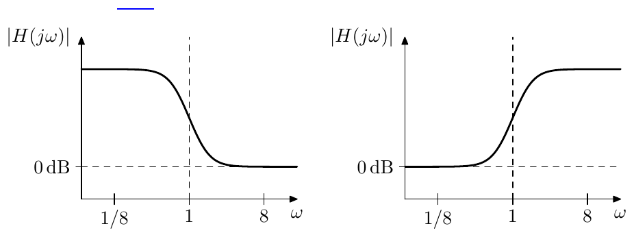
Figure 10.1: Shelving amplitude responses, ideally symmetric in fully logarithmic scale.
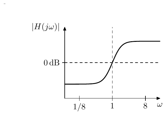
Figure 10.2: Tilting amplitude response, ideally symmetric in fully logarithmic scale.
Fig. 10.1 apparently shows low-shelving (left) and high-shelving (right) am- plitude responses. The amplitude response in Fig. 10.2 can be referred to as tilting amplitude response. It is easy to notice that the low- and high-shelving responses can be obtained from the tilting one by vertical shifts. Vertical shifts in decibel scale are corresponding to multiplication of the signal by a constant. That is tilting and low- and high-shelving filters can be obtained from each other by a multiplication by a constant. We will therefore not make much distinction between these types, arbitrarily jumping from one type to the other, whenever the discussion requires so.
Reciprocal symmetry of poles and zeros
Treating as the logarithmic origin of an amplitude response graph we can express the desired symmetry of the tilting amplitude response in Fig. 10.2 as an odd logarithmic symmetry:
Construction as a lowpass ratio2
Let be a filter (now this is a different than we have been using above) having the following properties: doesn’t have zeros, all its poles are lying on the unit circle, and .
Apparently, is a lowpass filter, which should be obvious by considering the factoring of into a cascade of 1- and 2-poles. Such also can be factored as
(where the leading coefficient is 1 due to being real stable, , and ). The poles of lying on the unit circle and being conjugate symmetric imply the reciprocal symmetry of the poles: if is a pole of then so is .
Let’s apply the cutoff substitution (, ) to . We obtain
That is we obtain the filter with the poles . Respectively, shifting the cutoff in the opposite direction by the same logarithmic amount, we have
That is we obtain the filter with the poles .
Since for each there is , for each there is . That is, the poles of are mutually reciprocal with the poles of and we can construct
By construction the poles of are the zeros of and the poles of are the poles of . Thus the poles of are reciprocal to its zeros and vice versa. However generally (a little bit later we’ll show that ). This means that is not a tilting filter, but is related to the tilting filter by some factor. Noticing that , we conclude that must be a kind of high-shelving filter. The conversion to the tilting filter is trivial: we can simply divide the result by .
The conversion to the low-shelving filter looks more complicated, since ap- parently and we have a 0/0 uncertainty evaluating . However we can notice that at we have , and , thus , that is simply . We therefore obtain the low-shelving filter from the high-shelving one by dividing by .
We can also obtain the explicit expression for the value of , where we can simply use the symmetries of the amplitude response. Since is a tilting filter, it must have mutually reciprocal amplitude responses at and , that is
from where and . Thus the tilting filter is obtained from the high-shelving one by dividing by .
Therefore we have
for the high-shelving, tilting and low-shelving filter respectively. From the values , , obtained earlier for the high-shelving filter we thus obtain:
Apparently can be greater or smaller than 1, corresponding to increasing or decreasing of the signal level in the respective range. Since and are filter cutoff factors, must be positive.
The filters constructed by the lowpass ratio approach satisfy the symmetry (10.5), however we know little about the shapes of their amplitude responses. These shapes can be arbitrary odd functions (if seen in the logarithmic scale), whereas we would like to obtain the shapes at least resembling those in Figs. 10.1 and 10.2.
Also, apparently the lowpass ratio approach can be easily applied to a But- terworth , since Butterworth (unit-cutoff) filters have poles on the unit circle. On the other hand, while EMQF filters also have poles on the unit circle, they don’t have only poles, but also zeros, therefore this method is not directly applicable to EMQF filters.3 In order to have a better control of the amplitude responses and to be able to build tilting and shelving filters based on EMQF filter, we will need to address the problem from a different angle.
Construction by mixing
We have already made some attempts of constructing a low-shelving filters by mixing the lowpass signal with the input signal, which weren’t too successful. Instead we could attempt the same mixing in terms of squared amplitude re- sponse, in which case we at least would not have the effects of the phase response interfering. Also, rather that constructing a low-shelving filter, we shall attempt to construct a tilting filter, in which case it is easier to express the symmetry requirement (10.5).
Suppose is defined by
We construct the tilting squared amplitude response by mixing with the squared “amplitude response of the input signal”, which is simply 1:
where and (or, equivalently, and ) denote the unknown positive mixing coefficients. We wish to satisfy (10.5).
Assuming a lowpass , that is for and for , we notice that and , therefore (10.5) can be attained only at and we can drop one of these variables obtaining:
However there apparently are additional restrictions on which ensure that (10.5) holds for any and not just for and . To find these restrictions let’s substitute (10.9) into (10.5):
and
The equation (10.10) thereby ensures that (10.5) will hold.
Let , or . Then (10.10) becomes4
while (10.9) becomes
That is, we simply want satisfying (10.11). Then (for any arbitrarily picked ) will satisfy (10.10) and respectively will satisfy (10.5).
Comparing the above to the lowpass-ratio approach to the construction of the tilting filters, that is comparing (10.12) to (10.6) we notice obvious similar- ities. Essentially (10.12) is a ratio of two lowpasses :
with an additional gain of , which occurs since this is a tilting rather than high-shelving filter.
Given a Butterworth , we have , that is the cutoff substitution is equivalent to choosing , in which case (10.12) means essentially the same as (10.6). The difference appears in the EMQF case where .
The zeros of the EMQF filter would have been exactly the problem in the case of (10.6), since the cutoff substitution also shifts the zeros, and the zeros of do not match the zeros of , respectively they cannot cancel each other in and would have resulted in zero amplitude response at the zeros of the numerator and in infinite amplitude response at the zeros of the denominator. On the other hand, in (10.12), where the EMQF zeros correspond to the poles of , the poles of will result in identical zeros of the numerator and of the denominator of , thus they will cancel each other. In that sense, the approach of (10.12) is more general than the one of (10.6).
We can also notice that the right-hand side of (10.12) monotonically maps the range of onto if and onto if . Since negating doesn’t have any effect on (10.12), therefore we can restrict to , in which case we can say is varying between and .
Obviously, (10.12) results in
The values at the key points respectively are (under the restriction )
where we also assume that and . In the EMQF case, where this is not true for even , and we need to understand (10.14) as referring to the points where and instead (which we didn’t explicitly write in (10.14) for the sake of keeping the notation short).
As with in the lowpass ratio approach, can be greater than 1 or smaller than 1.
10.3 Fixed-slope shelving
Using Butterworth filters as a basis for a shelving/tilting filter is compatible with both lowpass ratio (10.6) and mixing (10.12) approaches, where both options are giving equivalent results. For now we will continue the discussion in terms of the lowpass ratio option (10.6).
We will be interested in shelving filters obtained from the Butterworth filters of the 1st kind by (10.6). Noticing that (10.6) commutes with the Butterworth transformation:
we can restrict our discussion to the shelving filters obtained by the application of (10.6) to the 1st-order Butterworth lowpass. By (10.15) higher order shelving filters will be simply Butterworth transformations of the 1st-order Butterworth shelving filters, which is going to be covered in Section 10.5.
Since the 1st-order Butterworth lowpass coincides with the ordinary 1-pole lowpass, we simply have
and respectively by (10.7)
By (10.8)
Implementation
The 1st-order tilting filter can be implemented as a linear combination of the lowpass and highpass signals:
where the cutoff of the 1-pole multimode is at . The low- and high- shelving filters can be obtained from the above mixture by a division a or mul- tiplication by :
Amplitude response
The example amplitude responses of the 1-pole tilting filter are presented in Fig. 10.3, where the formal “cutoff” frequency is denoted as , being the middle frequency of the tilting.
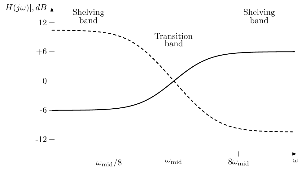
Figure 10.3: Amplitude responses of a 1-pole tilting filter for (solid) and (dashed).
Since the amplitude response of the tilting filter neither decreases to zero anywhere, nor does it have a range where it is approximately unity, we can’t define pass- and stop-bands. Instead we can refer to the bands on the left and on the right, where the amplitude response is almost constant, as shelving bands. The band in the middle where the amplitude response is varying can be referred to as transition band, as usual.
On the other hand, for low- and high-shelving filters we can define one of the bands, where the amplitude response is approximately unity, as the passband (Figs. 10.4, 10.5).
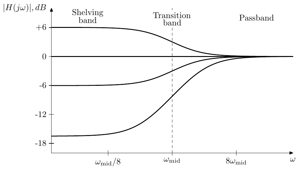
Figure 10.4: Amplitude responses of a 1-pole low-shelving filter.
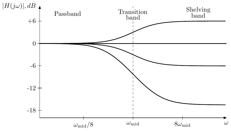
Figure 10.5: Amplitude responses of a 1-pole high-shelving filter.
Phase response
The representation of the shelving filter as a ratio of two lowpasses with cutoffs and allows an intuitive derivation of the tilting filter’s phase response, the latter being equal to the difference of the lowpass phase responses:
(since both shelving filters and the tilting filter all have identical phase responses, we picked the one with the most convenient transfer function).
Recalling how the phase response of a 1-pole lowpass looks (Fig. 2.5) we can conclude that the biggest deviation of the tilting filter’s phase response from (potentially reaching almost ) should occur in the frequency band between and , the deviation being positive if and negative if . Outside of this band the phase response cannot exceed . Fig. 10.6 illustrates. Notice that therefore the phase response is close to zero outside of the transition region.
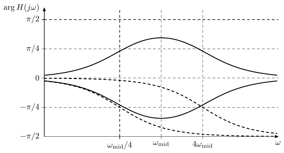
Figure 10.6: Phase response of the 1-pole shelving/tilting filters for (positive) and for (negative). Dashed curves represent phase responses of the underlying 1-pole lowpasses at cutoffs and .
Transition band width
In order to roughly estimate the width of the transition band of the tilting filter’s amplitude response we could divide the decibel difference in amplitude response levels at and by the derivative of the amplitude response at the middle of the transition band (Fig. 10.7).
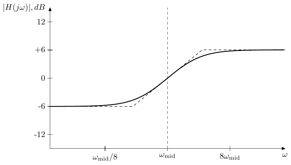
Figure 10.7: Estimation of the transition bandwidth of the 1-pole tilting filter by approximating the amplitude response by a broken line tangential to the amplitude response at the middle frequency.
Writing out the derivative of the amplitude response in the logarithmic frequency and amplitude scales (where we use natural logarithms to simplify the math), we obtain
(where we have assumed throughout the entire transformation chain). The logarithmic amplitude difference is and thus the bandwidth in terms of natural logarithmic scale is the ratio of that difference and the derivative at :
Introducing the natural-logarithmic amplitude boost , we rewrite the above as
where
is the “cardinal hyperbolic tangent” function, introduced similarly to the more commonly known cardinal sine function .
Introducing the decibel difference betwen the right and left “shelves”
we can switch the amplitude scale from natural logarithmic to decibel:
Then
Switching from the natural logarithmic bandwidth to the octave bandwidth we have
and we have obtained the octave bandwidth formula:
The graph of the dependency is plotted in Fig. 10.8. At we have . At we have , that is the bandwidth is growing proportionally to the decibel boost.5 Since the shelving boosts are typically within the range of dB, or maybe dB, we could say that the typical transition band width of the titling filter is roughly 3 octaves.
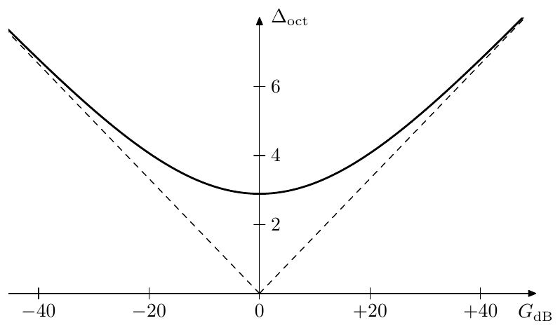
Figure 10.8: Transition bandwidth (estimated) as a function of the total decibel boost.
10.4 Variable-slope shelving
With shelving filters based on Butterworth filters of the 1st kind we didn’t have any control over the steepness of the transition slope, or, respectively over the transition band width. In order to introduce that kind of control we can use Butterworth filters of the 2nd kind.
The commutativity relation (10.15) still applies, since it’s independent of whether the involved filters are 1st or 2nd kind Butterworth, and we can restrict our discussion to the 2-pole shelving filters. Shelving filters of higher (even) orders can be obtained from those by Butterworth transformation, which is going to be covered in Section 10.5.
A generic unit-cutoff 2-pole lowpass filter
has its poles on the unit circle, no zeros and unity gain at , thus the requirements of the lowpass ratio approach are fulfilled and we can obtain the respective shelving filters by (10.7):
where by (10.8)
Implementation
In order to construct an implementation of the tilting filter, we simply express its transfer function in terms of the SVF modes:
where the cutoff of the multimode SVF is (notice that we used the normalized bandpass mode instead of the ordinary bandpass). Respectively
Amplitude and phase response
Notably, defined by (10.16) cannot be conveniently expressed in terms of (9.18), since
Respectively, (10.12) doesn’t apply and we cannot use the associated interpretation to reason about the shelving amplitude response shapes obtained from . However, we could notice that at the filter turns into a squared 1st-order Butterworth, while at it turns into a 2nd-order Butterworth of the 1st kind, therefore we can apply the results of Section 10.3 concluding that at least at these values of we should expect to obtain a resonable shelving shape.
The family of amplitude responses of a 2-pole tilting filter for various is shown in Fig. 10.9. One can see in the picture that controls the slope, or equivalently, the width of the transition band, however only a small range of generates “reasonable” tilting curves. We’ll analyse this topic in detail a bit later.
The phase response expressed in terms of a lowpass ratio gives
(where ). Recalling the 2-pole lowpass phase response (Fig. 4.6) we can conclude that the biggest deviation of the 2-pole tilting filter’s phase response from (potentially reaching almost ) should occur in the frequency band between and , the deviation being positive if and negative if . Outside of this band the phase response cannot exceed . Fig. 10.10 illustrates. Notice that thus the phase response is close to zero outside of the transition region.
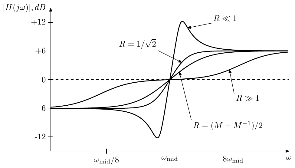
Figure 10.9: Amplitude responses of a 2-pole tilting filter for and various .
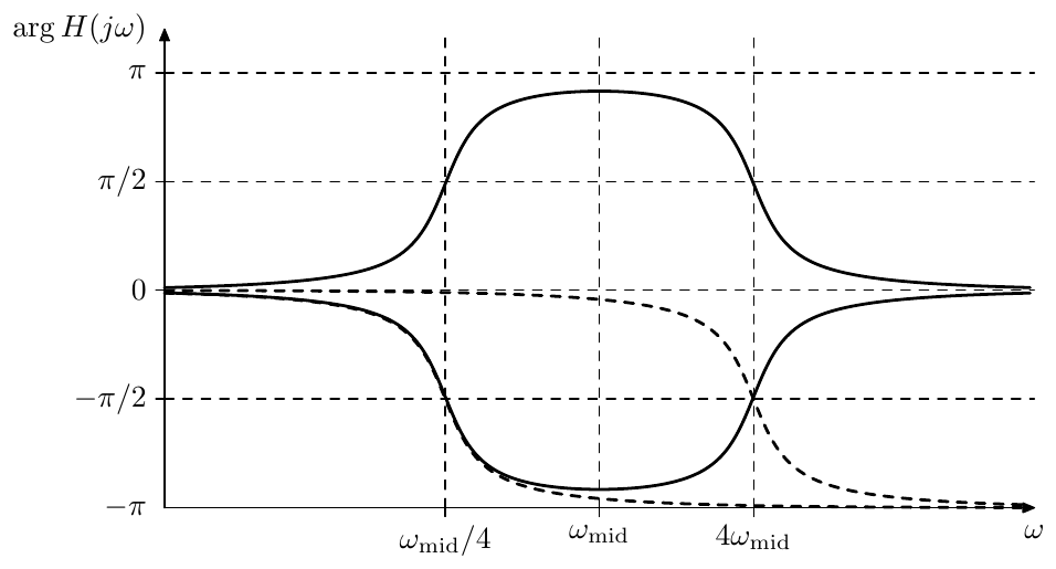
Figure 10.10: Phase response of the 2-pole tilting filter for (positive) and for (negative). Damping . Dashed curves represent phase responses of the underlying 2-pole lowpasses at cutoffs and .
Steepness control
As one could notice from Fig. 10.9, the damping parameter affects the steepness of the amplitude response slope at . Let’s analyse it in more detail. First, we write as
where
Then, considering the derivative of the fully logarithmic-scale amplitude response at , we obtain (assuming thoughout the entire transformation chain):
The maximum possible value is attained at and is equal to
That is, we can’t reach infinite steepness. Further, as one can see from Fig. 10.9, for the amplitude response gets a peak and a dip, which are generally undesired for a shelving EQ.
On the other hand, given a sufficiently large , we can attain arbitrarily small steepness. However, for the filter falls apart into a product of two 1-pole tilting filters.6 As grows, the 1-pole cutoffs get further apart and one can see the two separate “tilting inflection points” in the amplitude response (Fig. 10.9).
We need therefore to restrict to “a reasonable range”. But how do we define this range? Let’s analyse several characteristic values of .
At we have a two times vertically stretched (in the decibel scale) amplitude response of the 1-pole tilting filter with the same cutoff :
It should be no surprise that at we obtain a Butterworth transform of the 1-pole tilting filter with cutoff :
We can also obtain the response identical to the response of the just mentioned 1-pole tilting filter with cutoff by combining such 1-pole tilting filter with a “unit-gain” (fully transparent) tilting filter :
Therefore, such response is attained at .
Thus we are having two good candidates for the boundaries of the “reasonable range of ”. One boundary can be at , corresponding to the amplitude response of the 1-pole tilting filter with cutoff , the other boundary is at , corresponding to the same response shrunk horizontally two times.7 The steepness at therefore varies by a factor of 2 within that range, which also can be verified explicitly:
These boundary responses of the “reasonable range of ” can be found among the responses shown by Fig. 10.9.
10.5 Higher-order shelving
Butterworth shelving of the 1st kind
Given a 1-pole tilting filter:
we have reciprocal “cutoffs” in the numerator and the denominator. Respectively, the zero is reciprocal to the pole. According to (8.12c) and (8.12d), this property is preserved by the Butterworth transformation. The dampings of the poles and zeros obtained after the Butterworth transformation of the 1st kind depend solely on the transformation order and thus are identical in the numerator and denominator:
Therefore we obtain a serial chain of 1- and 2-pole tilting filters. The low- and high-shelving filters are transformed similarly. Alternatively we can simply reuse the obtained Butterworth transformation of the tilting filter, multiplying or dividing it by the factor .
Notice that the factor being rather than is a kind of a notational difference. After the Butterworth transformation of -th order the original change of cutoff by the factor will turn into a change of cutoff by the factor. Raising to the -th power (according to (10.8)) to obtain the multiplication factors gives .
Butterworth shelving of the 2nd kind
Remember that the “cutoffs” of the numerator and denominator of a 2-pole tilting filter are mutually reciprocal, while the “dampings” are equal:
so the numerator “cutoff” is and the denominator “cutoff” is .
By using the Butterworth transform cutoff property (8.12c) we obtain that must have the following form:
which is in agreement with the reciprocal cutoff preservation property of the Butterworth transformation. Thus we have obtained a serial chain of 2-pole tilting filters with numerator “cutoff” and denominator “cutoff” . The low- and high-shelving filters can be transformed similarly or obtained from the transformed tilting filter.
Wide-range slope
Let be a 2-pole tilting filter. In the discussion of the 2-pole shelving filters we mentioned that such filter smoothly varies its response from the one of a 1-pole shelving filter to as varies from to :
where the steepness of the amplitude response respectively doubles on that range.
Now let initially be equal to and imagine we have smoothly decreased it to . Suppose at this moment we swapped the 2-pole tilting filter with a 4-pole tilting filter simultaneously resetting the damping back to . Using (10.18) we have
and thus this swapping doesn’t change the frequency response of the filter. Now we can vary from to again to smoothly double the amplitude response once more.
So it seems we have found a way to vary the steepness of the tilting filter by a factor of 4 without getting the unwanted amplitude response artifacts which occur in a 2-pole tilting filter on an excessive range of . However the problem is the swapping of with and back. In mathematical notation the swapping is seamless, because the transfer function doesn’t change during the swap. In a real implementation however the swapping means replacing one filter structure with another and this will generate a transient, unless the internal states of the two filters are perfectly matched at the moment of the swapping.
Recall, however, that at the 2-pole can be decomposed into two 1-poles, where the second of the 1-poles is fully transparent:
Applying Butterworth transformation of order to both sides we obtain
This means that we could have a 4-pole filter
(where and are 2-pole sections) all the time. As long as we are interested in a 2-pole response we let
As we are switching from to neither of the sections is changed. From this point on we can further change from to updating the coefficients of according to .
This procedure can be repeated again, that is, having reached for the 4-pole shelving response, we can replace by
simultaneously resetting to . The idea is the same, we decompose into
and we let
until the point of the switching from to where we start having
Of course the same procedure can be further repeated as many times as desired (keeping in mind that the order of the resulting filter grows exponentially). Thus we can choose some power of 2 as a maximum desired filter order and switch this filter’s response from to to etc. each time reaches . The steepness of the amplitude response thereby smoothly varies by a factor equal to the filter’s order.8
Another way of looking at this is noticing that, as the response steepness grows, we are traversing the responses defined by , , , etc. Therefore we can consider this as if it was a smooth variation of the Butterworth tilting filter’s order.9
10.6 Band shelving
The 2-pole bandshelving filter can be easily obtained by applying the LP to BP substitution to the 1-pole low-shelving filter. Or, we can apply the LP to BP substitution to the 1-pole tilting filter (obtaining a kind of a “band-tilting” filter) and multiply the result by the necessary gain factor.
Let’s do the latter. Given
we perform the substitution
obtaining
where the SVF damping is equal to , where is determined by the bandwidth of the LP to BP transformation. The obtained filter could be referred to as “band-tilting” filter (Fig. 10.11).
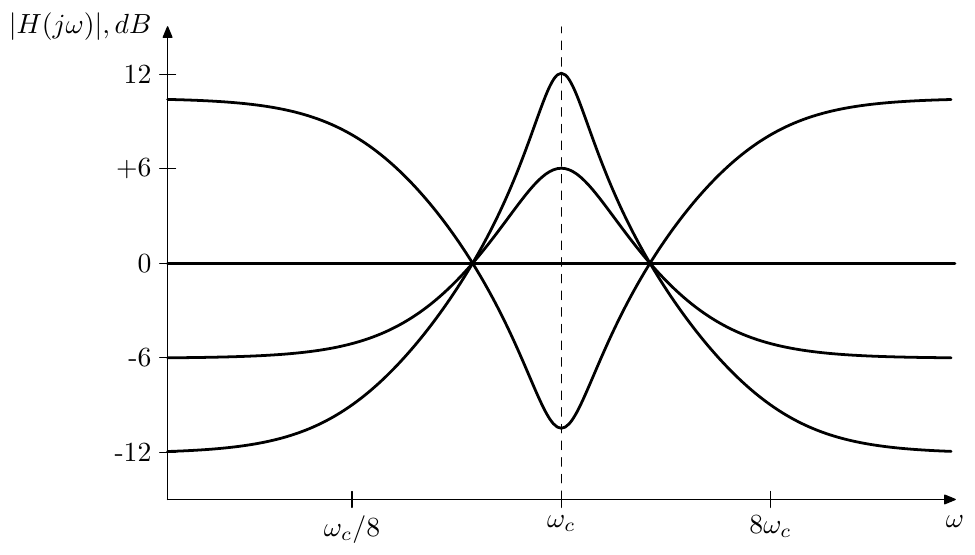
Figure 10.11: Amplitude response of 2-pole band-tilting filter for various .
In order to turn this filter into the band-shelving filter, apparently, we have to divide the response by :10
(mind that the SVF damping is still being equal to ). Thus, the 2-pole band-shelving filter can be implemented by mixing the (normalized) bandpass signal to the input signal. The amplitude response at the cutoff is which thereby defines the shelving gain. The desired bandwidth of the shelving can be achieved using the properties of the LP to BP substition, namely the formula (4.20).
It is interesting to observe that the above band-shelving transfer function can be rewritten as
that is we have a ratio of two filters with different dampings and , where the filters themselves could be lowpass, highpass or bandpass (the important thing being that they have identical numerators, which then cancel each other).
Band shelving of higher orders
The band-shelving Butterworth filter of the 2nd kind is obtained by applying the Butterworth transformation to the 2-pole band-shelving filter (10.19):
Thus we have a ratio of two 2nd order polynomials both having unit cutoff but different damping. Applying the Butterworth transformation we therefore obtain a cascade of 2nd-order sections with unit cutoff:
Apparently each such 2nd-order section is a 2-pole bandshelving filter with the shelving boost and the bandwidth defined by the parametrs and . Fig. 10.12 shows the amplitude response.
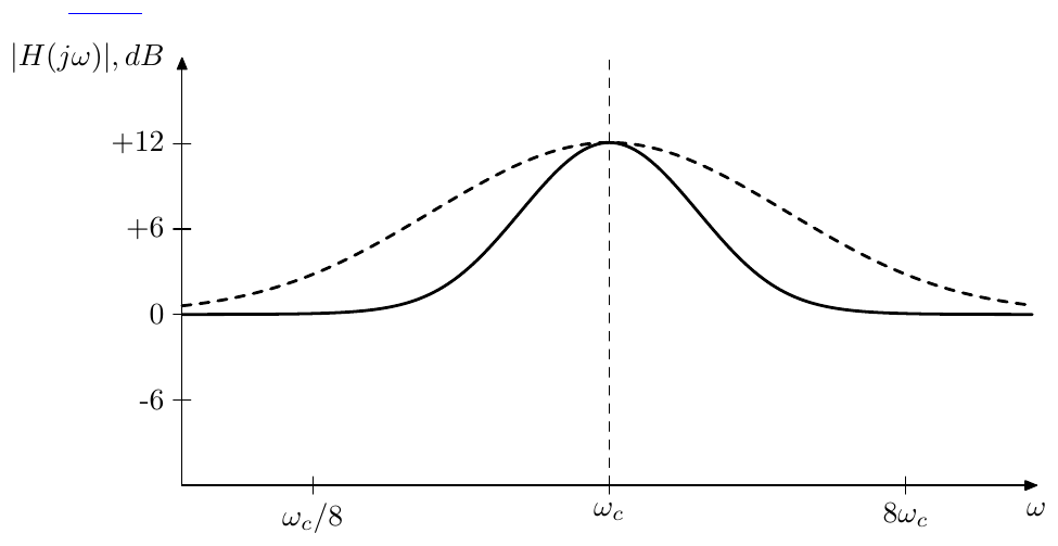
Figure 10.12: 4th order band-shelving Butterworth filter of the 2nd kind vs. 2nd order band-shelving filter (dashed line).
Another kind of band-shelving filter can be obtained by applying the LP to BP substitution to a Butterworth low-shelving filter of the 2nd kind. A useful feature of this approach is that by choosing the order of the low-shelving filter (and thus choosing the steepness of the low-shelving filter’s slope) one can choose the steepness of the slopes of the band-shelving filter.
10.7 Elliptic shelving
We have mentioned that the mixing approach of (10.12) can be applied to EMQF filters. Of all equations (10.13) it’s probably easiest to use (10.13a) to construct a high-shelving filter, the other filters can be derived from it in a trivial way. As (10.13a) is a monotonic mapping of the range of onto the range of contained between 1 and , we are going to have smoothly varying from 1 to as varies from 0 to , just with some ripples in the pass and shelving bands.
Letting in (10.13a):
we obtain the amplitude response shown in Fig. 10.13. Notice that due to the monotonic nature of the mapping (10.13a) the pass and shelving band ripples do not oscillate around the reference gains 1 and (corresponding to and ), but are rather occurring “into the inside” of the range between 1 and .
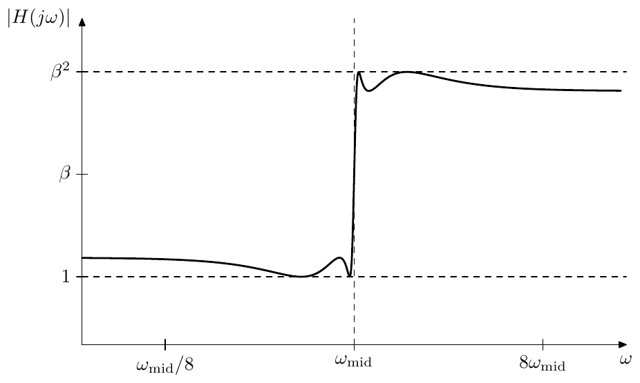
Figure 10.13: Amplitude response of an elliptic high-shelving filter. Horizontal dashed lines denote the reference gains 1 and .
Implementation
From (10.20) we obtain the pole and zero equations for :
where we ignore the poles of , since they cancel each other within anyway. The equations (10.21) are essentially identical to (9.152), where we let and or respectively.11
Having obtained the poles and zeros we can define the leading gain coefficient of the cascade form (8.1) from the requirement
We could also use a simpler requirement:
however we should mind the possibility of accidentally obtaining a phase response at .
Control parameters
In order to compute the passband () ripple amplitude, we can notice that in the passband the value of varies between 0 and . By (10.20) the maximum deviation from the reference gain 1 will be at the gain equal to
thus in the passband varies between 1 and . If then and vice versa. By the reciprocal symmetry (10.5) the deviation from the shelving band’s reference gain is the same, just in the opposite direction, thus in the shelving band varies between and .
From (10.22) it’s easy to notice that reciprocating reciprocates and vice versa. Therefore without loss of generality, for the sake of simplicity we can restrict the discussion to , , in which case the passband ripples occcur within and the shelving band ripples occur within . The case of , will follow automatically, where the ripple ranges will be and respectively.
Recall that the value of grows simultaneously with , where the latter is defining the elliptic transition band . Thus we are having three user-facing parameters, each of those being independently related to its respective variable:12
Transition bandwidth: Shelving gain: Ripple amplitude:
where the dependency between the three variables is given by (10.22).
Apparently at fixed the value of grows with and vice versa. At fixed , the value of grows with and vice versa. At fixed , the values of and change in opposite directions. Thus, if e.g. we want a smaller transition band, this means we want larger and larger , which means larger (given a fixed ). This means there is a tradeoff between the transition bandwidth (which we usually want small) and the ripple amplitude (which we also usually want small). There are similar tradeoffs between the other two pairs of the user-facing parameters.
Given any two of the three parameters, we can find the third one from (10.22). The explicit expressions for and can be obtained by transforming (10.22) to
from where on one hand
(where apparently the restriction is ), on the other hand
(where will ensure ) and can be obtained by (9.138).
At the formula (10.24) doesn’t work, since the amplitude response of is simply a horizontal line at unity gain and any of the values of will do. Respectively at the formula (10.23) doesn’t work, since must be equal to 1 in this case.
Notably, since (10.22) works equally well for and , so do (10.23) (under the restriction ) and (10.24) (under the restriction ). In practice the numerical evaluation of (10.23) for could raise concerns of potential precision losses, therefore it’s better to apply (10.23) to the reciprocal value of , which is larger than 1, and then reciprocate the result once again.
Steepness control
As with 2nd kind Butterworth shelving filters, we would like to be able to estimate the logarithmic midslope steepness of the elliptic shelving filter. Evaluating the following derivative at , by (10.20) we have
Recalling the formulas (9.145), (9.150) and Fig. 9.61, we find that, as expected, steepness grows with and . Unfortunately, differently from the 2nd kind Butterworth case, the expression (10.25) (or, specifically, (9.145)) is not easily invertible as a function of , which means we cannot easily find from the desired slope steepness. However, for each given this function’s inverse can be tabulated and we could use the midslope steepness instead of transition bandwidth as a control parameter.
Centered ripples
If we allow equiripples in the pass and shelving bands, it would be reasonable to require that these equiripples are not unipolar but rather centered around the required reference gains of these bands. We are going now to derive the respective formulas, which will be slightly simpler to do in terms of the tilting filter:
where again, for simplicity of discussion, without loss of generality we will assume , .
As a first step, we shall define the new reference gains, corresponding to the logarithmic centers of the equiripples. Since the left shelving band ripples occur within , their logarithmic center is at . Similarly, since the right shelving band ripples occur within , their logarithmic center is at . Therefore we introduce and the new reference gains and at the logarithmic centers of the equiripple ranges (Fig. 10.14).
We want to use instead of as one of the three control parameters. Since the entire framework of elliptic shelving filters has been developed in terms of , and , we’ll need to be able to convert from to . At the first sight this seems to be trivially done by , however this can be done only if we know .
Recall that we have three control parameters , and but only two freedom degrees, which means that we can specify only two of the three parameters, while the third parameter needs to be found by the respective relations. Similarly, if the three control parameters are now , and , we are going to specify only two of them. So, if we specify and , then indeed we can simply find and then find by (10.24). Specifying and is apparently the same as before and doesn’t pose any new probleems. However there is yet an option of specifying and , in which case we need to find either or , so that the other variable can be found from (10.23) or (10.22).
Let’s find . Substituting the equation (10.22) into we obtain
Similarly to (10.23), formula (10.26) also works for , , but due to numeric reasons in this case it’s better to apply it to the reciprocal and then reciprocate the result.
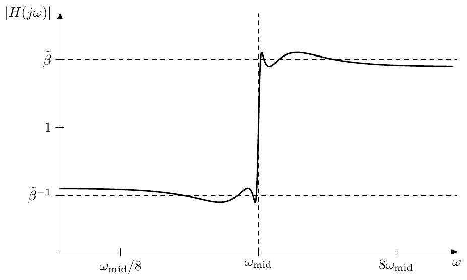
Figure 10.14: Centered reference gains and of an elliptic tilting filter.
Thus we have developed a way to express the tilting filter in terms of the centered reference gains and by converting from to either by or by (10.26). For the high- and low-shelving filters one needs to additionally take into account that the new reference gains imply different multiplication factors for conversion from tilting to the respective shelving factors:
so that the centered passband reference gain is at 1 and the centered shelving reference gain is at or respectively.
Relation to Butterworth shelving
At we have and the elliptic shelving filters turn into respective 1st-kind Butterworth shelving filters. However also notice that a 2nd-kind Butterworth shelving filter of order at is equal to the 1st-kind Butteworth shelving of the same order, which in turn is equal to the elliptic shelving filter of the same order at . That is at and all three kinds of shelving filters coincide.13
In that sense elliptic shelving can be seen as another way of extending the 2nd-kind Butterworth variable-slope shelving into the range beyond . Instead of reducing below (which would result in one large resonance peak in each of the pass and/or shelving bands), we could switch to the elliptic filter parameters14 obtaining a number of smaller equiripples. This particularly means that in the wide-range slope technique described in Section 10.5 instead of increasing the filter order at we could switch to elliptic equations (if we are willing to accept the ripples).
At however there is essentially no difference between 2nd-kind Butterworth shelving at and elliptic shelving, except for different formal control parameters. Indeed, both filters have two poles and two zeros which are mutually reciprocal and are also having conjugate symmetry. This leaves only two degrees of freedom, one degree corresponds to choosing the cutoff of the poles (which simultaneously defines the cutoff of the zeros as the reciprocal value of the poles cutoff) the other degree being the damping of the poles (which simultaneously defines the damping of the zeros as both dampings must be equal). However the first degree of freedom is taken by controlling the shelving gain and the second degree of freedom is taken by varying the or the parameter respectively. Thus the difference between the two filters can be only in how the control parameters are translated to the transfer function and in the leading gain coefficients of the transfer functions (where we would have in the Butterworth case and in the elliptic case).
Combining with other techniques
Elliptic design of shelving filters can be combined with other design techniques. Particulary, we can apply the LP to BP transformation to an elliptic low-shelving filter to obtain an elliptic band-shelving filter.
In principle one also could apply Butterworth transformation to elliptic filters to increase the slope steepness. However, since we are already having ripples in the pass and shelving bands, it would be more efficient to simply increase the order of elliptic filter, thereby attaining higher slope steepnesses (compared to applying the Butterworth transformation) at the same ripple amplitude.
10.8 Crossovers
Sometimes we would like to process different frequency bands of a signal differently. In the simplest case we would want to split the signal into low- and high-frequency parts, process one of them or both in some way and then merge them back (Fig. 10.15). This kind of filters, splitting the signal into different frequency bands are called crossovers.

Figure 10.15: The crosssover idea.
In principle we could take any a pair of lowpass and highpass filters to build a crossover, but some combinations would work better than the others. Particularly, imagine that the processing of different bands changes the signals very slightly, or sometimes maybe even doesn’t change them at all. In that case it would be really nice if the original signal was unaltered by the structure in Fig. 10.15, that is . However, this naturally expected property will not be given for granted.
Suppose we use a multimode 1-pole as a crossover basis, in which case the low- and high-pass filters share the same cutoff. Without loss of generality we could let (in other words, the crossover frequency will be at ):
Adding low- and high-pass transfer functions we have
Thus, if the low- and high-pass signals are unmodified by the processing, adding them together at the end of the network in Fig. 10.15 would restore the original signal exactly.
However the same doesn’t hold anymore for 2-poles:
in which case we have
In fact, as we may recall, the above is a notch filter. Of course, we could add the missing bandpass component, e.g. splitting it equally between the low- and high-bands:
but then the rolloff of the resulting low- and high-pass filters becomes 6dB/oct instead of former 12dB/oct, leading to the question, why using such 2-pole in the first place when a 1-pole would have done similarly.
Butterworth crossovers
If we relax the requirement of the sum of unprocessed signals being exactly equal to the original signal and allow a phase shift in the sum, while retaining the amplitudes, we essentially require that the low- and high-passes should add to an allpass:
Let’s take (1st kind) Butterworth low- and high-passes at the same cutoff :
where is the filter order and denotes the common denominator of and . Remember that the denominator is defined by the equation
while all roots of must lie in the left complex semiplane.
Adding the low- and high-passes together we obtain
Assuming is odd, for we get
Notably, the same property holds for the difference of Butterworth low- and high-passes of odd order
For an even order however becomes purely real for
and we get either a zero at if the above gets the form , or, if it gets the form then
Apparently the expression in parentheses is symmetric in logarithmic scale around and attains a minumum at this point, respectively attains a maximum, which we can evaluate by substituting , obtaining . Respectively thus the amplitude response of has a +3dB bump at .
As both and share the same denominator, they can be implemented by a single generalized SVF (the controllable canonical form in Fig. 8.1) using the modal outputs for the numerators 1 and respectively. Alternatively one could use multimode features of the serial cascade representation. Parallel representation is also possible, where we would pick up different modal mixtures of the same parallel 2-poles as the low- and high-pass signal respectively.
Linkwitz-Riley crossovers
If instead of Butterworth lowpass and highpass filters we take squared Butterworth filters:
(notice the conditional inversion of the squared highpass signal) we do obtain a perfect allpass for any :
and thus, since is Hermitian, . A crossover designed in this way is referred to as Linkwitz-Riley crossover. Since the denominators in (10.27) are identical, we again can use a shared structure, such as a generalized SVF or a multimode serial cascase to produce the output signals of both and . The parallel representation is problematic, since we are now having repeated poles due to the squaring of the denominators.15
Note that the phase responses of and are identical, since the phase contributions of their numerators are zero, while the phase contributions of their denominators are identical. This in-phase relationship of the split bands is the key feature of Linkwitz-Riley crossovers16 (contrary to the somewhat common opinion that the key feature of Linkwitz-Riley crossovers is the absence of the +3dB bump, which, as we have seen is also e.g. the case with odd-order Butterworth crossovers).
The in-phase relationship actually also includes :
Indeed
where we used the Hermitian property of .
Generalized Linkwitz-Riley crossovers
The Linkwitz-Riley design consisting of two squared Butterworth filters is a special case of a more generic idea which we will discuss below.17
First we need a kind of auxiliary lemma. Let be a real polynomial of . We now state that the formal frequency response is real nonnegative if and only if can be written in the form , where is some other real polynomial of . The proof goes like follows.
Suppose . Then for
Conversely, suppose . Since is simultaneously real and Hermitian, it must be even, and so must be . Therefore it can be factored into . Let’s chose to contain the left complex semiplane roots of , thereby will contain the right complex semiplane roots. If has roots on the imaginary axis, these roots will all have even multiplicities (since otherwise will be changing sign at these points) and therefore we can split these roots into two identical halves, which we assign to and respectively. Since is real, its poles are conjugate symmetric and so will be the poles of and .
We still need to show that the leading coefficient of will be real. Let denote the leading coefficient of . Then the leading term of is . By substituting we obtain the leading term of , which is . However the coefficient of the leading term of must be positive, otherwise would become negative at large . Since is positive, is real. That completes the proof.
Now, given two real polynomials and with real nonnegative frequency responses, we can construct a third real polynomial as their sum
Since the frequency responses of and are nonnegative, so is the frequency response of . By the previous discussion, the above equation can be rewritten as
Dividing both sides by the right-hand side, we obtain
We wish to interpret the two terms in the left-hand side as transfer functions. However, these functions are not stable, since the roots of are lying in the right semiplane. We can however multiply both parts by :
thereby making both filters stable and turning the right-hand side into an (also stable) allpass. Also notice that the orders of and do not exceed the order of , therefore the terms of (10.31) are nonstrictly proper rational functions of , as required for transfer functions of (integrator-based) differential filters. Introducing
we rewrite (10.31) as
and thus we have built a crossover (provided is a kind of a lowpass and is a kind of a highpass). Again, the denominators are identical and we can use a shared structure for and .
Notice that (10.33) is simply (10.28) divided by . The phase responses of all terms of (10.28) are apparently zero, therefore the phase responses of all terms of (10.33) are identical and simply equal to :
The identical phase responses, as we should remember, are the key feature of Linkwitz-Riley crossover design, thus we have built a kind of generalized Linkwitz-Riley crossover.
The identical phase responses of , and also allow to rewrite (10.33) in terms of amplitude responses:
It is often convenient to define
By (10.32), where . Apparently and therefore (10.34) turns into
The interpretation in terms of and suggests another, somewhat more practical approach to building generalized Linkwitz-Riley crossovers. We start with a pretty much random filter , although satisfying , so that (10.35) can hold. From and , using (10.32), we obtain and and can simply find as . In principle, the obtained can be used as it is, but we can also further factor it into thereby obtaining .18 Of course, in order for and to count as a “reasonable” crossover, must be a lowpass or lowpass-like filter (which can be ensured by choosing a lowpass- like ), and the obtained must be highpass-like. Or the other way around.
Alternatively we might be able to simply “guess” and (or, equivalently, and , or and ). E.g. the previously discussed Butterworth filter-based Linkwitz-Riley crossover arises by choosing to be a Butterworth lowpass and to be a Butterworth highpass, which gives , and respectively , . The same result is obtained by by choosing , (respectively and ). This gives (10.29) in the form
from where
where is the Butterworth denominator. The equation (10.31) respectively takes the form
which is essentially the same as (10.27).
Symmetric generalized Linkwitz-Riley crossovers
Ideally in (10.33) we would like to have symmetric amplitude responses
as it was e.g. the case with Butterworth-based Linkwitz-Riley crossover. Apparently (10.36) is not guaranteed for an arbitrary pair of and which satisfies (10.33) (where satisfying (10.33) is understood in the sense that the sum of and is an allpass). We would like to find a way of obtaining generalized Linkwitz-Riley crossovers satisfying (10.36).
Recall that (10.35) is just another intepretation of the crossover equation (10.33). On the other hand, compare (10.35) to (10.4). By (10.4), the equation (10.35) will be satisfied by and related through an LP to HP transformation, if , where is the function used to construct by (9.18).
This is not sufficient yet, as besides satisfying (10.35) (and respectively (10.33)), we need to have the same poles in and , so that they can share the same denominator . However we have already shown that and will have the same poles if .
Therefore, in order to obtain a generalized Linkwitz-Riley crossover with symmetric amplitude responses, we need to take obtained from satisfying and .
EMQF Linkwitz-Riley crossovers
We already know one function satisfying : the normalized elliptic rational function . Therefore EMQF filters might be a good candidate for symmetric generalized Linkwitz-Riley crossovers. Notice that at EMQF filters turn into Butterworth filters and we obtain a classical (Butterworth-based) Linkwitz-Riley crossover.
Therefore let be an EMQF (lowpass) filter and be the respective highpass. Recall that the zeros of elliptic lowpass filters are positioned on the imaginary axis in pairs symmetric relatively to the origin, with the exception of the zero at the infinity, which occurs if the order of the filter is odd. Therefore can be written as
which means that . Respectively can be written as
where the factor arises from the zero of occuring at the infinity which turns into a zero of occurring at the origin. Therefore .
Therefore , and (10.33) takes the form
Fig. 10.16 shows the example of amplitude responses of and .
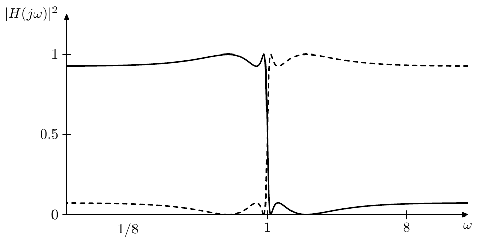
Figure 10.16: Amplitude responses of EMQF crossover low- (solid) and high-pass (dashed) outputs.
Centered ripples
Next we will describe a way to further improve the amplitude response of generalized Linkwitz-Riley crossovers. The techniques can be applied to pretty much any generalized Linkwitz-Riley crossover, but for the sake of simpler presentation we’ll be using the EMQF crossover as an example.
Recall that the phase responses of , and are identical. Let be this common phase response. Then we can introduce the zero phase frequency response functions
Notice that since , we have
That is we can consider , and as amplitude response functions.
We are now going to construct some linear combinations of the above zero phase frequency responses. Since they are all related to the original frequency responses via one and the same factor , linear combinations of , and correspond to exactly the same linear combinations of , and . E.g.
We can think of these linear combinations as of linear combinations of amplitude responses, resulting in the new amplitude responses, with the reservation that the new “amplitude responses” may become negative (which in terms of true amplitude responses would have been interpreted as changing the phase response by ).
Consider that the passband ripple amplitude of is , while the stopband ripple amplitude is . Respectively the passband ripples of and oscillate within , while the stopband ripples oscillate within , which corresponds to the absolute maximum deviations from the ideal values of 1 (passband) and 0 (stopband).
Note that so far the deviations are unipolar. The deviation from 1 occurs towards zero, while the deviation from zero occurs towards 1. We could make these deviations bipolar instead, simultaneously reducing the maximum deviation. The (linear) midpoints of the oscillation ranges are for the stopband and for the passband. We can take the range between these middles and stretch it to This can be achieved by the transformation
which should be applied to both lowpass and highpass:
Thereby the deviation amplitude is multiplied by , but simultaneously the deviations become centered around the ideal values 0 and 1, which effectively halves the deviations. Thus the deviation amplitude is effectively multiplied by becoming equal simply to (Fig. 10.17).
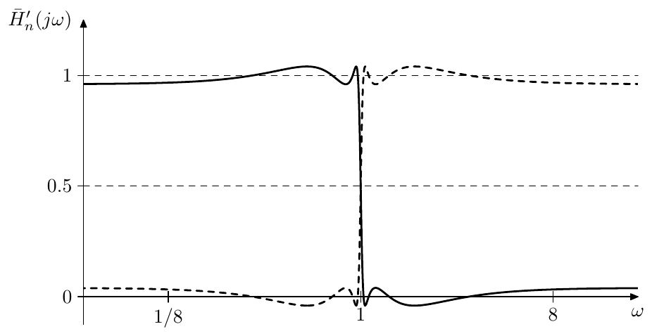
Figure 10.17: Zero-phase frequency responses of adjusted EMQF crossover low- (solid) and high-pass (dashed) outputs.
Multiplying the above equations by we obtain the same transformation for and :
Note that thereby we still have
Phase correction
If we need to do some processing in parallel to the crossover, then we should keep in mind that the crossover signals are phase shifted, therefore it could be a good idea to introduce the same phase shift into the signal which bypasses the crossover.
At this point we will assume that the crossover is (generalized) Linkwitz- Riley, therefore all phase shifts are identical. In this case the simplest way to construct a phase-shifted bypass signal is by adding the LP and HP outputs of the crossover together, which by the previous discussion should be an allpass signal with exactly the same phase shift as in LP and HP signals (Fig. 10.18). Notice that the LP and HP outputs of the crossover in Fig. 10.18 correspond to the and transfer functions in (10.33). Particularly, if we’re using a Butterworth or an EMQF crossover, the squared HP signal needs to be inverted for odd .
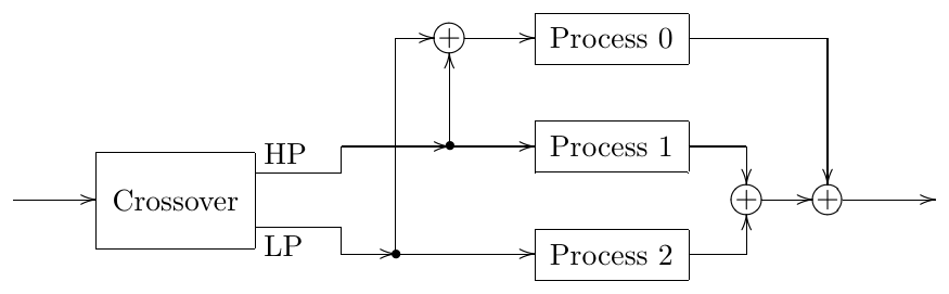
Figure 10.18: Adjusting the phase of the bypass signal.
The approach of Fig. 10.18 doesn’t work if the bypass signal processing path is not starting from the same point where the crossover is connected. In this case we might need an explicit phase-correction allpass. Fig. 10.19 shows the option of doing the phase correction prior to the processing of the bypass signal.
Rather than constructing the correction allpass following the idea of Fig. 10.18 (that is building such an allpass as another crossover with LP and HP outputs added), it is more efficient to construct this allpass directly. Indeed, by (10.32), given a crossover whose order is , the order of the allpass is only . Therefore it is more efficient to implement the correction allpass simply as an -th order filter:
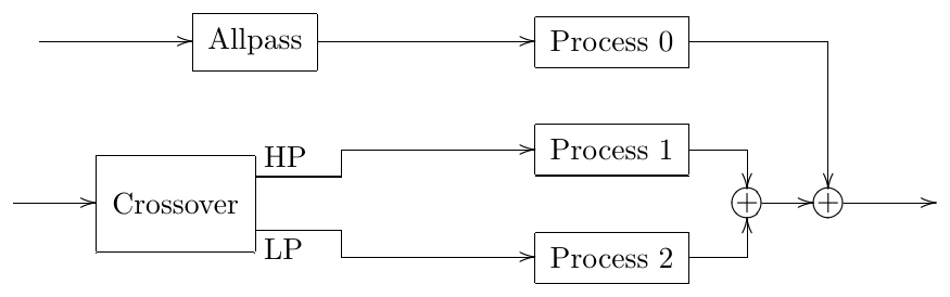
Figure 10.19: Adjusting the phase of the signal from a different source.
In Fig. 10.19 we could swap the order of the phase correction and the processing of the bypass signal as shown in Fig. 10.20. If the processing is nonlinear, this may result in an audible change in the sound. One could argue that the option shown in Fig. 10.20 is better, since the nonlinear processing is done on the original signal, while the allpass correction of the processing results would be usually inaudible (unless another nonlinear processor is following), and thus the bypass processing would sound pretty much identical to the one in the absence of the phase shifts. However, there is a counterargument that all other processing is done on phase-shifted signals, and it would be more consistent to do the same for the bypass signal.
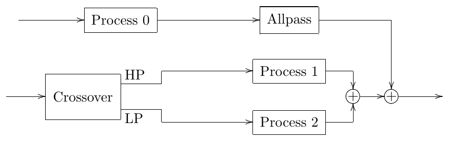
Figure 10.20: Correction allpass at the end of processing.
A more complicated situation arises if we want to stack the crossovers to make a multiband crossover because in this case the phase correction is needed even if there is no bypass signal. Consider Fig. 10.21, where denotes an allpass introducing the phase shift corresponding to the crossover . The LP and HP outputs of the crossover are completely in-phase, therefore the signal going through the processor is, from the phase shift perspective, essentially the same as bypass signal of the crossover and thus needs phase correction equivalent to the phase contribution of . Or, looking from a slightly different angle, the input signals of processors and contain phase shifts from both crossovers, while the input signal of processor contains the phase shift only from the first crossover and thus needs an additional phase shift by .
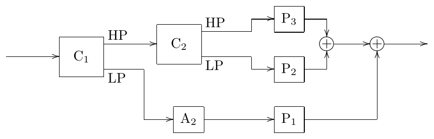
Figure 10.21: Phase correction in 3-way crossover mixing.
If the bypass signal processing is present, we could modify the structure of Fig. 10.21 as shown in Fig. 10.22. An alternative option is presented in Fig. 10.23 and yet another option (requiring one more corection allpass) in Fig. 10.24. Notice that Fig. 10.22 does all phase shifting at the beginning and Fig. 10.24 does all phase shifting at the end, while the structure in Fig. 10.23 is a kind of in-between mixture of Fig. 10.22 and Fig. 10.24. These ideas generalize by induction to higher numbers of bands, where in Fig. 10.22 we’ll be adding new crossover-allpass pairs on the left, whereas in Fig. 10.24 we would be adding crossovers on the left and allpasses on the right.
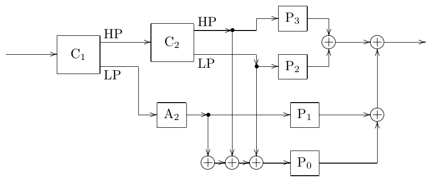
Figure 10.22: Phase correction of bypass signal in 3-way crossover mixing.
In four-way crossover mixing there are new options, e.g. there is a symmetric band splitting option shown in Fig. 10.25. However practically it is not much different from the approach of Fig. 10.22 generalized to 4 bands, since the total phase shifts in the input signals of all processing units contain the total sums of the phase shifts associated with all crossovers in either case.
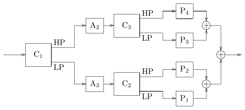
Figure 10.25: Symmetric 4-way crossover.
Note that in Fig. 10.25 one could also wish to replace the allpasses and with a single allpass in one of the paths, which just corrects the difference between the phase responses of and . This is however not possible. Indeed, assuming identical orders of and , their phase responses are identical at each of the points and . Therefore the phase response of must be equal to zero at both and . But this is not possible for a differential allpass.19 The argument becomes somewhat more complicated if the crossovers are allowed to have different orders, where one would need to consider the factored forms of and , essentially reaching the same conclusion.
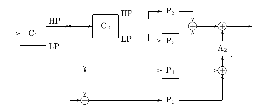
Figure 10.23: Another way of phase correction of bypass signal in 3-way crossover mixing.
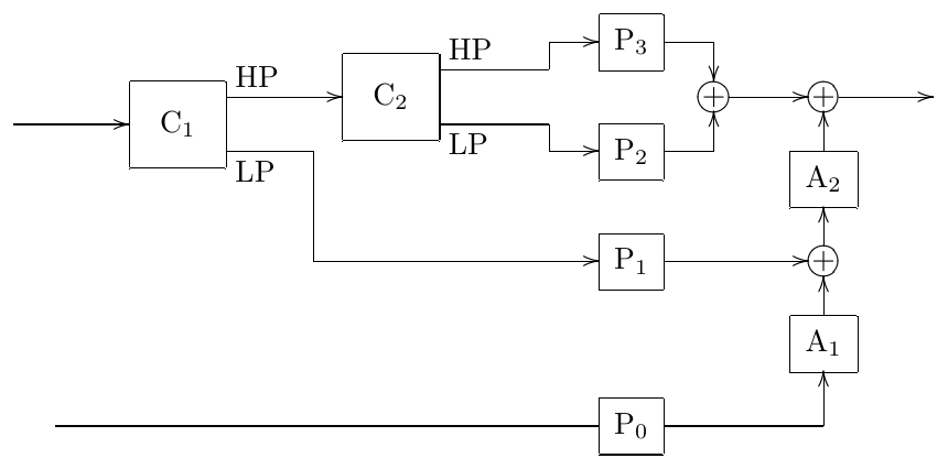
Figure 10.24: 3-way crossover mixing with all phase correction done at the end.
10.9 Even/odd allpass decomposition
Suppose we are given a filter defined by (9.18). In this section we are going to show that is expressible as a linear combination of the “even” and “odd” allpasses, that is allpasses based on the even and odd poles of .
Recall that we have defined even poles as solutions of (or equivalently ) and odd poles as solutions of (or equivalently ). Let’s introduce the following notation:
that is the product is being taken over all left- or respectively right-semiplane even poles of in the first two lines, and over all even poles of in the third line. We will also use , and with similar meanings for the respective products based on the odd poles of . We also introduce
where goes over all poles of , or, equivalently, over all zeros of .
In this notation we could express the construction of from its poles and zeros as
where denotes a placeholder for the yet unknown gain coefficient, which we then find from the requirement of to have a specific value at some point on the imaginary axis, and where denotes the value of at and so on. In the simplest case we will let , which gives , however we will also need to be able to take other choices of .
Now let’s introduce the “even” and “odd” allpasses:
where the gains and are defined by the conditions and :
(note that allpasses defined in this manner can be trivially built as cascades of 2nd- and 1st-order sections). The allpass property of and follows from the fact that is a real function of , therefore the even an odd poles of (which are respectively the solutions of and ) are mutually conjugate in terms of , that is they are symmetric with respect to the imaginary axis in terms of . Figs. 8.11, 8.12 and other similar figures illustrate.
Apparently both and are stable filters. If additionally is an odd function and , then and are real. Indeed, suppose , that is is an even pole. Then is also an even pole since
The same can be shown for odd poles. Therefore the poles of each of the and are mutually conjugate and, since , both fiilters are real. If is not an odd function, particularly if is even, then the poles of and do not have the conjugate symmetry, therefore and are essentially complex filters. However this shouldn’t be a problem, since we will use and only as intermediate transformation helpers.
Now we attempt express as a linear combination of and . Consider the obvious algebraic relationship:
where . Equation (10.39), if interpreted in terms of , can be understood as a relationship between three transfer functions, the two transfer functions and in the left-hand side adding up to the doubled transfer function in the right-hand side. The poles of these transfer functions are identical20 and consist of the full set of the even poles of .
By analysing the behavior of these transfer functions for we also notice that the two functions in the left-hand side of (10.39) are allpasses, while the transfer function in the right-hand side has an amplitude response identical to . So, amplitude response-wise (10.39) is already what we are looking for and we just need to correct it so that it also becomes what we want transfer function-wise.
Let’s multiply (10.39) by :
Considering the product in the right-hand side of (10.40) we have
Comparing to (10.37) we notice that we essentially have obtained . Matching the values at to find (and remembering that ) we obtain
Considering the second term in the left-hand side of (10.40) we obtain
Comparing to (10.38a) we notice that we essentially have obtained . Matching the values at we obtain
Thus (10.40) turns into
or
Thus we have represented as a linear combination of and .
If and is an odd function, then . Thus we obtain and and therefore (10.41) turns into
If the order of is even, then generally and the coefficients of the linear combination (10.41) are complex. Note that forcing or choosing another such that in this case doesn’t help, since the allpasses themselves are still complex. However, as we already mentioned, this won’t be a problem for our puproses.
10.10 Analytic filter
Sometimes in signal processing we want to deal with the so called analytic signals, which are defined as signals whose Fourier spectrum doesn’t contain any negative frequencies (that is the amplitudes of the negative frequency partials are all zero). Since spectra of real signals must be Hermitian, apparently analytic signals can’t be real, thus they are essentially complex.
Occasionally there is a need to convert a real signal into an analytic signal by dropping all of its negative frequency partials. This is very similar to the lowpass filtering, except that this time we want to dampen not the frequencies but the frequencies . Such filter can be referred to as analytic filter. The process of removing the negative frequencies from a real signal is also known as the Hilbert transform, for that reason the analytic filter is probably more commonly known under the name Hilbert transformer.
The opposite conversion is simple: we just take the doubled real part of the analytic signal. That is, given an analytic signal we can restore the original signal by
This effectively turns each complex partial of the form to a real partial , which can be equivalently seen as adding a negative frequency partial .
Construction from a lowpass
The basic idea of constructing an analytic filter is simple, we take a unit-cutoff lowpass filter (so that the passband is and the stopband is ) and rotate its transfer functions along the imaginary Riemann circle:
This effectively rotates the frequency response along the real Riemann circle:
thereby transforming the passband to and the stopband to (Fig. 10.26).
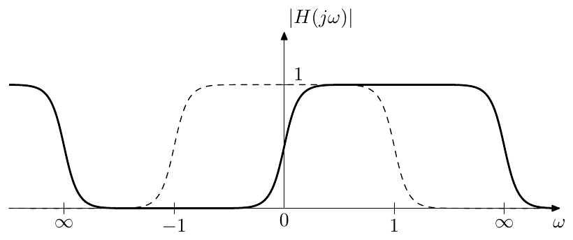
Figure 10.26: Conversion of a unit-cutoff lowpass filter into an analytic filter by a rotation of the real Riemann circle.
The poles and zeros of are respectively transformed by the inverse of , which is . Therefore the poles and zeros of can be explicitly obtained from the poles and zeros of by , . The gain coefficient of can be found by equating the frequency responses of and at corresponding frequencies, e.g. . Note that in principle, we can multiply by an arbitrary complex number of unit magnitude, as this wouldn’t change the amplitude response of . Particularly, we could let .
Parallel allpass implementation
In practical implementation we usually don’t want to deal with complex signals. In this case the output of the filter is a fundamentally complex signal, so we can’t avoid that. However we could try to construct as much as possible of staying in real signal domain. Particularly we could attempt to express using real filters, where we then do some postprocessing by mixing the real outputs of those filters with possibly complex coefficients. This is indeed possible.
Suppose is implemented using (9.18). Recall that by (10.41) the lowpass filter can be represented as a linear combination of allpasses. This linear combination must be preserved by the rotation in (10.43) giving
Since rotates along the imaginary axis (in terms of plane and its respective Riemann sphere), the allpass property should be preserved by this transformation and and must still be allpasses. It would be convenient to reexpress and in terms of their new poles after the transformation by .
As mentioned, the poles are transformed by . Therefore let’s introduce the new allpasses
where and are defined from the conditions , . Apparently,
where denote two different yet uknown coefficients. Substituting into the above we find that these coefficients must be simply equal to and respectively and therefore
Up to this point we have been explicitly keeping the freedom of choice of . This has been done on purpose, as now we can see a good choice for . By letting we have and and thereby
or
Equation (10.44) would be an acceptable answer, provided and are real filters. Since and by construction, we only need to make sure that the poles of each of the and are conjugate symmetric.
Recall that the poles of and are obtained by . We therefore wonder, what would be the relationship between the two preimages of a conjugate pair of poles . Considering visually the effect of on the Riemann sphere, we could guess that . Verifying algebraically:
Therefore, given that poles of have the conjugate reciprocal symmetry (that is, if is a pole of then so is ), the poles of and will have the conjugate symmetry.
The poles of will have the conjugate reciprocal symmetry, given that is a real function such that . Indeed, suppose and . Then
We already know one specific kind of lowpass filter where has such reciprocal symmetry: the EMQF filter (with the Butterworth filter as its limiting case). Note that EMQF poles not only have conjugate reciprocal symmetry, but are simply lying on the unit circle, in which case conjugate reciprocation simply maps the poles to themselves: . Since maps the unit circle to the real axis, the poles are real. Also, since is a rotation in the direction of the imaginary axis, it maps left semiplane poles to the left semiplane poles and thus . Thus, we are having stable real and whose poles are also all real.
Real and imaginary allpasses
The expression (10.44) can be simplified a bit further. Notice that for an EMQF filter we are having where is the filter’s order. Respectively . Therefore (10.44) turns into
Recall that we can multiply by any unit-magnitude complex number without changing the amplitude response. Particulary, we could multiply it by obtaining
Thus the real and imaginary parts of the output signal of are obtained completely separately from two parallel allpasses and .
10.11 Phase splitter
There is another, conceptually completely different, but closely mathematically related approach to constructing the Hilbert transformer. Considering a single positive-frequency complex sinusoidal partial
we notice that the imaginary part of the signal is phase-delayed by relatively to the real part. Now let denote the analytic filter operator. That is, applying discards the negative frequency partials from the signal. Then, applying analytic filtering to we have
Respectively, for a general real signal we have
Introducing notations:
(where is the signal with all real sinusoidal partials phase-shifted by ) we have
Equation (10.46) gives us another approach to the implementation of the analytic filter: we take the halved original signal as its own real part, and phase shift the partials of its real spectrum by to obtain the imaginary part. Also notice that (10.46) is exactly the opposite of (10.42).
Differently from the approach in Section 10.10 where we didn’t care about the phase, the approach of (10.46) explicitly preserves the phase of the partials, thus (10.46) defines a zero-phase analytic filter. Unfortunately, as we shall see later, such filter cannot be implemented by a stable differential system. Still, the whole approach is somewhat more straightforward than the one of Section 10.10.
We will also develop a number of useful explicit expressions, which will be helpful in the construction of . In principle, the same expressions could have been derived in Section 10.10 (as the answers are essentially the same), however the derivations will be somewhat more direct in the context of the new approach.
Complex spectral form
Before we get to the construction of the phase shifter, we need to reexpress this phase shifting in terms of complex spectral partials:
That is we need to phase shift the positive frequency partials by and phase shift the negative frequency partials by . Since the amplitudes are unchanged by the phase-shifting, this is an allpass transformation, which we can denote by the operator:
Note that the fact that the negative frequencies need to be phase shifted by the opposite amount is in agreement with the fact that , being the imaginary part of , needs to be a real signal. Therefore needs to preserve the hermiticity of the spectrum of . This means that the frequency response of must be a Hermitian function, which implies the phase response being an odd function.
The frequency response of the allpass is obviously
We are still uncertain as to which value to assign to . In principle, according to (10.47) the zero-frequency partial should be completely killed in , thus
Strictly speaking, this kills the allpass property of at , but this is actually the only way to keep Hermitian.
Now we can rewrite (10.46) in the pure operator form
or in the frequency response form
The complex spectrum interpretation of (10.46) gives another insight into why does it describe an analytic filter. Given a positive-frequency complex sinusoidal signal we have and respectively
that is is unchanged by . On the other hand, if , then and respectively
The DC at is neither a positive- nor a negative-frequency partial. According to what we discussed above, it is killed by and thus
(where denotes a signal equal to 1 everywhere).
Rational phase shifting allpass
We are looking for an allpass filter whose frequency response is
Apparently can’t be a rational function, since rational functions are continuous everywhere except at their poles, where they gradually approach infinity, thus a rational function cannot accommodate a jump from to which has at . But we still can build a rational which approximates the ideal for .
As mentioned earlier, the ideal is an allpass everywhere except at . Since we are building an approximation of anyway, we can ignore that fact and build an approximation which is a perfect allpass. This will simplify our goal, since then we can construct the allpass in terms of its phase response. Therefore let
be the ideal phase response of our allpass.21 So, how can we build a rational allpass transfer function approximating ?
Consider the fact that the frequency response of an allpass can be explicitly written in terms of its phase response:
Using (9.11a) we can rewrite the same as
However , being a 1st-order rational function, maps rational functions to rational functions of the same order and back. Thus, if we have a rational function of some order such that
then and will also be rational functions of the same order and the phase response of will be equal to .
Letting we rewrite as
Will be a real function of ? Since must be real odd, so must be . This implies that it must be representable in the form where is some other real function. Therefore
and thus is real.
Before proceeding to the construction of we would like to give one warning. The allpass transfer functions , which will arise from the application of (10.52) to the obtained , will be unstable. This corresponds to the fact that phase responses of stable differential allpasses cannot stay around over a large range of .22 This is a fundamental limitation, which we’ll have to deal with. Later in this section we will describe a way of addressing this problem.
Construction of
The ideal is apparently
We wish to find a rational . This will ensure .
Let be a real rational function satisfying the unit-cutoff lowpass conditions (9.21). We would like to compose with other functions in such a way that the result is an approximation of . This composition should still result in a real rational function and, ideally, also preserve the order of . Therefore, good candidates for the elements of such composition are the rotations of real Riemann circle .
As a first step, we map the pass- and stop-band areas of (that is and ) to the areas where . This is achieved by (where the signs are matched). We thereby obtain which has the desired values in the “pass”- and “stop”-bands, however the bands themselves are incorrectly positioned on the argument axis, still coinciding with the pass- and stop-bands of a unit-cutoff lowpass. We could fix this by a real Riemann circle rotation of the argument. Which turns our candidate compositions into
where we initially treat the signs as independent.
However actually the signs in (10.53) cannot be independent. E.g. if we choose the “inner rotation” (the rotation of the argument of ) to be , this maps the original lowpass passband to . In this area we want , therefore we have to choose the “outer rotation” (the rotation of the value of ) to be as well. In a similar way we could choose both rotations to be . This means that the signs in (10.53) must be matched.
Intuitively it is clear that any “lowpass” kind of should result in (10.53) giving an approximation of . However we also need to be an odd function. Let’s see what kind of restriction this means for . By (9.13) the rotations map the odd symmetry to the reciprocal symmetry, which means that
which effectively brings us to the idea to use the EMQF function (or the Butterworth filter function as its limiting case).
Having chosen we can refine the formula (10.53) a little. Suppose we chose the “+” signs in (10.53). Then . Vice versa, if we choose the “” signs, then which is if is odd and if is even. In principle, this is not a very big problem, and both options are valid, but it would be just nice to have and respectively all the time. This is achieved by changing (10.53) into
The readers can convince themselves that (10.54) also gives an approximation of and that in this case regardless of . Fig. 10.27 illustrates.
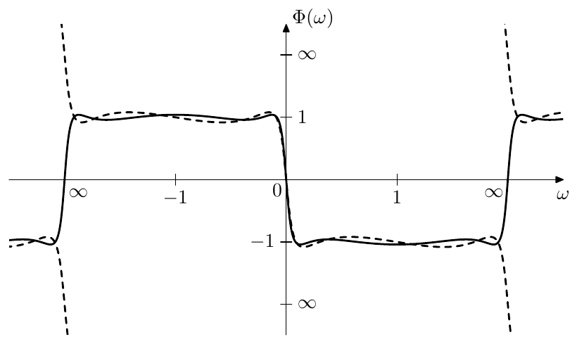
Figure 10.27: obtained from (10.54) and for even (solid) and odd (dashed) .
Explicit expression for EMQF
Sticking to the idea to use the EMQF function we will refer to the phase shifter that we are constructing as “EMQF phase shifter”. Even though this is some kind of a misnomer, this should provide a pretty clear identification of the approach we use.
Substituting into (10.54) we obtain
Since is a real rational function of order , so is .
In the real period-based preimage representation terms we have
Expressing (10.55) in the same terms we have
which by (9.111) turns into
Replacing with and with we obtain
and finally, switching to the explicit scaling form:
where and are the quarter periods corresponding to the elliptic moduli and , that is and are obtained by the double Landen transformation from and . Note that, since double Landen transformation solely changes the quarter period ratios and by a factor of 4, the degree equation (9.112) stays essentially the same: . Thus the imaginary periods of the two functions are matched, while the real period is scaled by .
Turning the representation form into the explicit form we obtain, e.g. using real period argument normalization
Expression (10.57) defines another (normalized) elliptic rational function. Differently from the already familiar , this function has equiripples around in the bands centered around . Strictly speaking the amplitudes of the upwards- and downwards-pointing ripples of (shown in Fig. 10.27) are not equal, rather, the values are mutually reciprocal at the upwards- and downward-pointing peaks. It is just that in arctangent scale the reciprocal values correspond to equal deviations from 1 or from . Therefore the true equiripple behavior occurs in the arctangent rather than linear scale. However according to (10.51) the function (which is our true goal) is exactly the arctangent scale representation of . Therefore will have true equiripples. For the sake of clarity we provide a graph of in Fig. 10.28, however notice that the only difference between Figs. 10.28 and 10.27. is the labelling of the vertical axis.
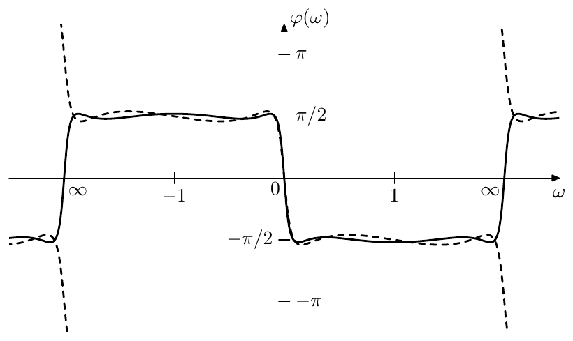
Figure 10.28: obtained from (10.57) and (10.51) for even (solid) and odd (dashed) .
Bands of EMQF
It is instructive to analyse in terms of its bands in the preimage domain. The readers can convince themselves that the bands are:
| Transition band 1 | ||
| Passband 1 | ||
| Transition band 2 | depends on | |
| Passband 2 |
where in the transition band 2 we have for even and for odd . Fig. 9.51 can be referred to as an illustration.
It is not difficult to realize that that the “passband” ripples of are essentially obtained from the ripples that the function has on the real axis (which thereby results in the upwards-pointing peaks being reciprocal to the downwards-pointing peaks) and on a parallel line which is away from the real axis by one half of its imaginary period. The details are left as an exercise to the reader.
Poles and zeros of EMQF phase shifter
We would like to construct from its poles and zeros. Since is an allpass, it is sufficient to find the poles, while the zeros can be trivially obtained from the poles. However we could also consider obtaining the zeros explicitly.
Starting with the equations and we apply the inverted (10.52), which is , yielding
where “” should be taken for poles and “” for zeros.
At this point there are different possibilities how to continue. Particularly, we could apply (10.55) which gives or equivalently . This would be pretty much the same as what we have been solving in Section 10.10.23 It could be more interesting and practical, though, to take a different path, which will allow us to obtain simple explicit expressions for the poles and zeros of . The obtained poles and zeros will be of course the same, since we are solving the same equations, just in a different way.
Let’s use the preimage representation (10.56) to solve (10.58), in a similar way to how we were solving the pole equations for other filter types. Recall that by the imaginary argument property, is essentially the same as , just rotated in its complex argument plane. Therefore, while was generating quasielliptic curves for its argument moving parallel to the real axis, will generate the same curves for its argument moving parallel to the imaginary axis. In order to solve (10.58), we would like the curves to go through , however the movement parallel to the imaginary axis in the preimage domain is not very useful for solving (10.58), since the imaginary periods are matched for the preimages of and , and therefore we will not obtain all possible solutions.
We should rather move parallel to the real axis. Apparently, in this case we won’t generate quasielliptic curves in the representation domain, but rather the kind of lines shown in Fig. 9.54. Since and respectively take each value only once within a quater-period grid cell, and since the values occur on horizontal lines where turns into or (Fig. 9.51), we need to move in one of these lines. The representation will then simply move along the imaginary axis24 in one and the same direction, looping through the point.
Choosing the horizontal line as the principal preimage line we have . We wish to have representation moving upwards along the imaginary axis therefore the preimages need to move towards the right (going along the line ). In terms of the same movement corresponds to moving along the line
where the direction of movement of is, obviously, also towards the right. Notice that any other possible choices of the principal preimage line of do not generate any additional solutions of (10.58), since will be simply traversing along the entire imaginary axis in any case.
The value moving upwards along the imagniary axis will be traversing the points at
where at even we’ll have and at odd we’ll have . That is, even correspond to zeros and odd correspond to poles. The values of are respectively
from where
from where by we obtain
where even correspond to zeros and odd correspond to poles. Note that in the Butterworth limit the equation (10.59) turns into
Since all values in (10.59) are real, the solutions given by (10.59) are also real. That is the poles and zeros of are real and can be factored into 1st-order allpasses.
Since the period of is , there are different values of given by (10.59). Half of them are zeros and the other half are poles, thus there are zeros and poles, where the poles and zeros are inverleaved (Fig. 10.29). Apparently, can run over any range of consecutive integers. A particularly convenient range is . In this case and give one pole/zero pair where the pole and the zero are mutually opposite. This pole/zero pair corresponds to the lowest-cutoff 1-pole allpass factor, which is stable since the pole is obtained from . The values and give another pole/zero pair corresponding to the next 1-pole factor, which is unstable since the pole is obtained from . The third 1-pole factor will be stable again etc.

Figure 10.29: Poles (black dots) and zeros (white squares) of an EMQF phase shifter for .
One could notice in Fig. 10.29 that there is reciprocal symmetry within the set of poles and zeros of . That is if is a pole or a zero of , then so is . Apparently, this is due to the property (9.74b) of the elliptic tangent function .
We could also derive a simple rule for remembering, whether for one obtains a pole or a zero, that is whether the closest to zero negative value of given by (10.59) is a stable allpass factor’s pole or an unstable allpass factor’s zero. First, notice that negating the allpass’s cutoff is equivalent to the substitution . Since the frequency response of a real filter is Hermitian, its phase response is odd, thus negating is equivalent to negating the phase response. Thus, since the phase responses of stable allpasses are decreasing, the phase responses of unstable (negative cutoff) allpasses are increasing. Now consider the phase shifter which is a product of stable and unstable allpasses. Intuitively, as starts to increase from 0, the phase response first has to decrease to approximately , therefore the allpass factor with the lowest cutoff in the chain must be stable.25
Bandwidth of EMQF phase shifter
In our discussion of the bands of EMQF we have established that the equiripple “passband” ranges are
that is
where we could notice that the logarithmic center of the “passband” is thereby at .
Respectively, the logarithmic bandwidth expressed in octaves is a logarithm base 2 of the ratio of the passband’s boundaries:
which gives us a way to immediately find from a given bandwidth:26
Since the boundaries of the bands of are identical to the bands of , the above formulas equally apply to the bands of .
The value of , which effectively defines the amplitude of the ripples, can be computed (after having constructeed ) from
However it is more practical to directly compute the deviation of from the target value (after having constructed ). According to the above formula, should be the point of maximum phase deviation (within the equiripple range) and thus the deviation of from should give the amplitude of the equiripples.
Since and increase or decrease simultaneously, will get larger ripple amplitudes for larger bandwidths and vice versa. Increasing the order will result in a smaller ripple amplitude for the same bandwidth.
Apparently the “passband” doesn’t need to be centered at and can be shifted to any other center frequency by the cutoff substitution . This raises a related question of prewarping, where we could notice that the situation is pretty similar to the prewarping of a normalized 2-pole bandpass filter (discussed in connection with the LP to BP transformation in Section 4.6). Therefore the suggested way of handling the prewarping of consists of the following steps:
- Given the desired “passband” :
prewarp its boundaries separately:
thereby obtaining the new prewarped “passband” of a different bandwidth and center frequency:
- Given the new bandwidth and assuming a unit center frequency, construct the allpass as previously described in this section.
- Apply the cutoff substitution to , which effectively means multiplying the cutoffs of the underlying 1-poles by the new center frequency .
This approach effectively implements an idea similar to the usage of a single prewarping point discussed in Section 3.8, which takes care of preserving the correct ratios between the cutoffs of the individual filters in the system. In principle it could be okay to prewarp each of the 1-pole factors of individually instead, however that apparently will somewhat destroy the optimality of the equiripple .
Phase splitter
Half (or approximately half, if is odd) of the poles of are unstable and we can’t implement directly. However, there is one trick which allows to work around this limitation. Before describing this trick we will switch the notation back from to to highlight the fact that the filter performs a phase shift (of the positive frequencies).
Let’s factor into a product of two allpasses:
where contains only the right-semiplane (unstable) poles and contains only the left-semiplane (stable) poles. As usual, we could assume or require that and , which is achievable, given and respectively .
Given a signal we wish to obtain the signal . Consider two other signals:
where . Notice that is a stable allpass and so is apparently , thus and can be obtained from by processing by stable allpasses and . Notice that
that is and are in a 90 phase shift relationship.
Apparently the same idea applies to arbitrary , which we can express in the operator notation as
where is the operator denoting the processing of a signal by the filter . Thus, even though we cannot phase-shift the input signal by 90, we can obtain two derived allpass signals and , where the phase difference between and is 90. Respectively, the combined signal
is an analytic version of , where the phase shift of this analytic version relatively to is defined by . The approach of generating two allpass signals which are in a 90 phase relationship is referred to as phase splitting and is illustrated in Fig. 10.30. Since is the real part of the analytic signal and is the imaginary part, the allpass produces the (doubled) real part and the allpass produces the (doubled) imaginary part and therefore we can refer to and as real and imaginary allpasses respectively.
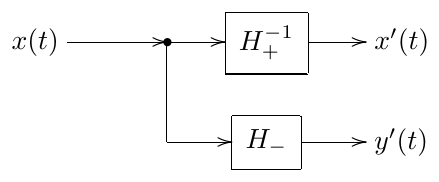
Figure 10.30: Phase splitter.
Notice that (10.61) is essentially the same as we have in (10.45), where and are corresponding to and (where which specific filter corresponds to which depends on the order ). Thus (10.45) also describes a phase splitter, just obtained from a different angle.
10.12 Frequency shifter
Even though frequency shifter is not a filter in the strict sense, its most critical part will be based around the Hilbert transformer, which is a filter. For that reason the discussion of frequency shifters may belong to the filter topic.
Suppose we are given a signal represented by its complex spectrum:
By multiplying the signal with a complex sinusoidal signal we effectively shift the frequencies of all partials by :
This is not very interesting, since given a real we obtain a complex . Obviously, it’s because we multiplied by the complex signal . In terms of signal spectra, the spectrum of was Hermitian, however by shifting the spectrum by we destroyed the Hermitian property.
However, this is also not exactly what we want if we think of frequency shifting. The complex spectrum is a more or less purely mathematical concept, while the one more intuitively related to our hearing of sounds is the real spectrum, and it’s the partials of the real spectrum whose frequencies we’d rather want to shift. That is, given
we wish to obtain
Notably, if , then some of the frequencies in (10.63) will be negative and will alias with the positive frequencies of the same absolute magnitude. This can be either ignored, or can be prefiltered to make sure it doesn’t contain frequencies below . So, except for the just mentioned highpass prefiltering option, the possible aliasing of the negative frequencies doesn’t affect the subsequent discussion.
We can rewrite (10.63) as
where
is a signal obtained from by phase-shifting all partials by . In the operator notation the same can be expressed as
We have already found out how to obtain a phase shifted signal in Section 10.11, except that we also found than such signal cannot be directly obtained. We will address this slightly later, while for now we shall take a different look at the same problem of frequency shifting.
Analytic signal approach
Looking again at (10.62) we can notice that the positive frequency partials are correctly shifted and it’s the negative frequency partials which make trouble. So, if the negative partials weren’t there in the first place:
we would have obtained
Comparing (10.66) to (10.63) we notice that they essentially consist of the same frequency partials, except that is missing the negative part of its spectrum. The negative part of the spectrum can be restored by (10.42), and thus (10.66) and (10.63) are related via
This is easier to see in the operator notation:
which is identical to (10.65), thus both approaches are equivalent.
Implementation
Let be the allpass from (10.60). Multiplying (10.65) by we obtain
If we are willing to accept the phase-shifted signal instead of (and as it seems, we don’t have much other choice) a frequency shifter can be simply implemented by the structure in Fig. 10.31.
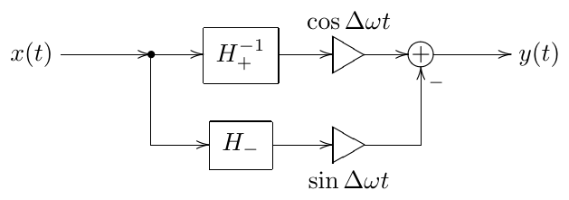
Figure 10.31: Frequency shifter.
Notably, replacing by in (10.67) we obtain
This means that we can extend the frequency shifter in Fig. 10.31 to a one that shifts simultaneously in both directions, obtaining the diagram in Fig. 10.32.27
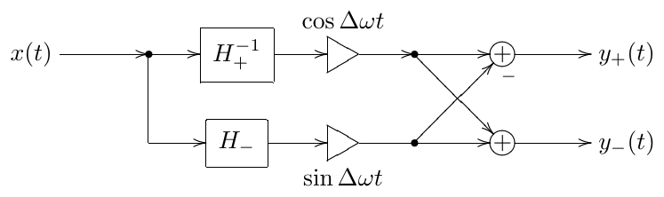
Figure 10.32: A bidirectional frequency shifter.
Adding together the frequency-shifted signals from (10.67) and (10.68) we notice that
or
That is, the sum of and in Fig. 10.32 essentially produces the ring modulation of by , except that the result of this ring modulation is doubled and phase-shifted by . So frequency-shifting and ring-modulation by a sinusoid seem are very closely related. The same can be analyzed in the complex spectral domain:
Thus in the case of the ring modulation by a sinusoid, the partials are frequency-shifted in both directions.
Aliasing
If then for some partials the sum may exceed the Nyquist frequency, respectively they will alias to (assuming unit sampling period ). This kind of aliasing is similar to the one occurring at in case of , however, while the aliasing around also occurs in the analog case, aliasing around Nyquist frequency is a purely digital phenomenon.
It is therefore up to the effect designer, whether the aliasing around should be prevented, or allowed. The aliasing at Nyquist is however usually undesired. It can be avoided by prefiltering the frequency band , which can be done by a lowpass filter with a cutoff around . Notice that is a discrete-time cutoff value and thus doesn’t need prewarping.
The aliasing around can be prevented in a similar way by using a highpass with a cutoff at (since in this case we assume , the cutoff will thereby be positive). Note that since the phase splitter has a limited bandwidth, one also may consider filtering out the signal outside that bandwidth anyway, regardless of .
10.13 Remez algorithm
The equiripple behavior of Chebyshev polynomials and elliptic rational functions is a characteristic feature of the so-called minimax approximations. , , , and the function used to build the phase splitter all provide specific analytic-form solutions to specific minimax problems. However, in a more general situation we might want a numerical solution approach.28
Suppose we are given a function and its approximation . There are different ways to measure the quality of the approximation. One way to measure this quality is the maximum error of the approximation on the given interval of interest :
We therefore wish to minimize the value of . That is we want to minimize the maximum error of the approximation. Such approximations are hence called minimax approximations.29
Gradient search methods do not work well for minimax optimizations. Therefore a different method, called Remez algorithm,30 needs to be used. As of today, internet resources concerning the Remez algorithm seem quite scarce, nor does this method seem to be a subject of common math textbooks. This might suggest that Remez algorithm belongs to a rather esoteric math area. The algorithm itself, however, is very simple. We will therefore cover the essentials of that algorithm in this book.31
Suppose is a polynomial:
Apparently, there are degrees of freedom in the choice of , each degree corresponding to one of the coefficients . Therefore we can force the function to take arbitrarily specified values at arbitrarily chosen points . Particularly, we can require
or equivalently require the error to be zero at :
(notice that the equations (10.71) are linear in respect to the unknowns and therefore are easily solvable). If the points are approximately uniformly spread over the interval of interest then intuitively we can expect to be a reasonably good approximation of (Fig. 10.33).
This based on the uniform zero spacing approximation is however not the best one. Indeed, instead let equal the (properly scaled) zeros of the Chebyshev polynomial of order :
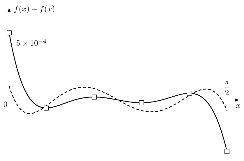
Figure 10.33: The error of the 4-th order polynomial approximations of on . The approximation with uniformly spaced zeros at , , , , (solid line) and the one with Chebyshev zeros (dashed line). The empty square-shaped dots at the extrema of the error are the control points of the Remez algorithm.
where the minus sign in front of the cosine ensures that are in ascending order. Comparing Chebyshev zeros approximation (the dashed line in Fig. 10.33) to the uniform zeros approximation, we can see that the former is much better than the latter, at least in the minimax sense.
A noticeable property of the Chebyshev zeros approximation clearly observable in Fig. 10.33 is that the extrema of the approximation error (counting the extrema at the boundaries of the interval !) are approximately equal in absolute magnitude and have alternating signs. This is a characteristic trait of minimax approximations: the error extrema are equal in magnitude and alternating in sign.
So, we might attempt to build a minimax approximation by trying to satisfy the equiripple error oscillation requirement. That is, instead of seeking to minimize the maximum error, we simply seek an error which oscillates between the two boundaries of opposite sign and equal absolute value. Somewhat surprisingly, this is a much simpler task.
Intuitive description of Remez algorithm
Consider the solid line graph in Fig. 10.33. Intuitively, imagine a “control point” at each of the extrema. Now we “take” the control point which has the largest error (the one at ) and attempt to move it towards the axis, reducing the error value at . Since there are 6 control points (4 at local extrema plus 2 at the boundaries), but only 5 degrees of freedom (corresponding to the coefficients ), at least one of the other control points needs to move (or several or all of them can move). Intuitively it’s clear that if we lower the error at , then it will grow at some other points of . However, since we have the largest error at anyway, we can afford the error growing elsewhere on , at least for a while. Notice that during such change the positions of control points will also change, since the extrema of the error do not have to stay at the same coordinates.
As the error elsewhere at becomes equal in absolute magnitude to the one at , we have two largest-error control points which need to be moved simultaneously from now on. This can be continued until only one “free” control point remains. Simultaneously reducing the error at 5 of 6 control points we thereby increase the error at the remaining control point. At some moment both errors will become equal in absolute magnitude, which means that the error at all control points is equal in absolute magnitude. Since the control points are located at the error extrema, we have thereby an equiripple oscillating error.
Remez algorithm for polynomial approximation
Given which is a polynomial (10.70), the process of “pushing the control points towards zero” has a simple algorithmic expression. Indeed, we seek which satisfies
where are the (unknown) control points (including and ) and is the (unknown) signed maximum error. Thus, the unknowns in (10.72) are (the polynomial coefficients), (the control points at the extrema) and (the signed maximum error). Notice that the equations (10.72) are linear in respect to and , which leads us to the following idea.
Suppose we already have some initial guess for , like the uniform zero polynomial in Fig. 10.33 (or the Chebyshev zero polynomial, which is even better). Identifying the extrema of we obtain a set of control points . Now, given these , we simply solve (10.72) for and (where we have equations and unknowns in total), thereby obtaining a new set of . In a way this is cheating, because are not the control points anymore, since they are not anymore the extrema of the error (and if they were, we would already have obtained a minimax approximation by simply finding these new ). However, the polynomial defined by the new has a much better maximum error (Fig. 10.34)!
So we simply update the control points to the new positions of the extrema and solve (10.72) again. Then again update the control points and solve (10.72) and so on. This is the Remez algorithm for polynomial approximation. We still need to refine some details about the algorithm though.
-
The function should be reasonably well-behaved (whatever that could mean) in order for Remez algorithm to work.
-
As a termination condition for the iteration we can simply check the equiripple property of the error at the control points. That is, having obtained the new , we find the new control points and then compute the errors . If the absolute values of are equal up to the specified precision, this means that we have an approximation which is minimax up to the specified error, and the algorithm may be stopped.
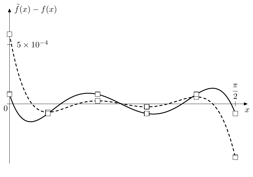
Figure 10.34: The approximation error before (dashed line) and after (solid line) a single step of the Remez polynomial approximation algorithm. The empty square-shaped dots are the control points.
-
The initial approximation needs to have the alternating sign property. This is more or less ensured by using (10.71) to construct the initial approximation. A good choice for (as demonstrated by Fig. 10.33) are the roots of the Chebyshev polynomial of order one higher than the order of the approximating polynomial .32
-
The control points are the zeros of the error derivative (except for and ). There is exactly one local extremum on each interval between the zeros of the error. Therefore, can be simply found as the zeros of the error derivative by bisection of the intervals .
-
After having obtained new , the old control points are not the extrema anymore, however the errors at are still alternating in sign. Therefore the new zeros (needed to find the new control points by bisection) can be found by bisection of the intervals .
Restrictions and variations
Often it is desired to obtain a function which is odd or even, or has some other restrictions. This can be done by simply fixing the respective , thereby reducing the number of control variables and reducing the number of control points and zero crossings accordingly.
Remez algorithm can also be easily modified to accommodate a weight function in the minimax norm (10.69):
The error function therefore turns into , while the minimax equations (10.72) turn into
(where is the reciprocal of ).
Remez algorithm for rational approximation
Instead of using a polynomial , better approximations can be often achieved by rational :
Besides being able to deliver better approximations in certain cases, rational functions can be often useful for obtaining approximations on infinite intervals such as , because by varying the degrees of the numerator and denominator the asymptotic behavior of at can be controlled.
For a rational defined by (10.73) the minimax equations (10.72) become nonlinear in respect to the unknowns and , although they are still linear in respect to the unknowns :
Notice that the number of degrees of freedom is now . The equations (10.74) can be solved using different numeric methods for nonlinear equation solution, however there is one simple trick.33 Rewrite (10.74) as
Now we pretend we don’t know the free term , but we do know the value of before the sum of :
where is this “known” value of . The value of can be estimated e.g. as the average absolute error at the control points . Then (10.75) are linear equations in respect to , and and can be easily solved. Having obtained the new and , we can obtain a new estimation for and solve (10.75) again. We repeat until the errors at the control points become equal in absolute value up to a necessary precision. At this point we can consider the solution of (10.74) as being obtained to a sufficient precision and proceed with the usual Remez algorithm routine (find the new , new etc.)
Here are some further notes.
-
In principle the solution of (10.74) doesn’t need to be obtained to a very high precision, except in the final step of the Remez algorithm. However, in order to know whether the current step is the final one or not, we need to know the true control points, so that we can estimate how well the equiripple condition is satisfied. Ultimately, this is a question of the computational expense of finding the new control points vs. computing another iteration of (10.75).
-
Sometimes, if the equations are strongly nonlinear, the trick (10.75) may fail to converge. In this case one could attempt to use the discussed below more general Newton-Raphson approach (10.81), where the damping parameter may be used to mitigate the convergence problems.
-
In regards to the problem of choice of the initial for the rational Remez approximation, notice that the zero error equations (10.71) take the form
which is fully linear in respect to and , and can be easily solved.
Other kinds of approximating functions
In certain cases one could use even more complicated forms of , which are neither polynomial nor rational. In the general case such function is controlled by a number of parameters :
(notice that this time the numbering of is starting at one, so that there are parameters in total, giving degrees of freedom). The minimax equations (10.72) become
Introducing functions
we rewrite the equations (10.76) as
Introducing vector notation
we rewrite (10.77) as
Apparently, (10.78) is a vector form of (10.72), except that now we consider it as a generally nonlinear equation. Both the function’s argument and the function’s value have the dimension , therefore the equation (10.78) is fully defined.
Different numeric methods can be applied to solving (10.78). We will be particularly interested in the application of multidimensional Newton-Raphson method. Expanding into Taylor series at some fixed point we transform (10.78) into:
where is the Jacobian matrix and . By discarding the higher order terms , the equation (10.79) is turned into
The equation (10.80) implies the Newton-Raphson iteration scheme
where the damping factor is either set to unity, or to a lower value, if the nonlinearity of is too strong and prevents the iterations from convergening. The initial value is obtained from the initial settings of the parameters and the estimated initial value of . As for the rational , the initial value of can be estimated e.g. as the average error at the control points.
Similarly to the rational approximation case, the solution of (10.78) doesn’t need to be obtained to a very high precision during the intermediate steps of the Remez algorithm. However the same tradeoff between computing the iteration step (10.81) and finding the new control points applies.
The choice of the initial can be done based on the same principles. The zero error equations (10.71) turn into
(notice that compared to (10.77) we have set to zero and we have rather than equations). Letting
we have an -dimensional nonlinear equation
which can be solved by the same Newton-Raphson method:
10.14 Numerical construction of phase splitter
For the sake of a demonstration example we are now going to use Remez algorithm to build an approximation of the ideal allpass phase shifter defined by (10.50), while deliberately staying away from the entire framework of elliptic functions. The obtained results shall be identical to the ones previously obtained analytically.
We will retain the mentioned allpass property in the approximation, therefore let denote the allpass which should approximate the ideal phase shifter (10.50). Using serial decomposition, can be decomposed into series of 2- and 1-pole allpasses. Since we aim to have with as flat (actually, constant in the range of interest) phase response as possible, 2-poles seem to be less useful than 1-poles, due to steeper phase responses of the former (Figs. 10.35 and 10.36).
Restricting ourselves to using just 1-poles we have:
where are the cutoffs of the 1-pole allpasses . Notice that the specific form of specifying in (10.83) ensures , that is we wish to have a rather than phase response at .
Now the idea is the following. Suppose in (10.83) (that is we have no 1-pole allpasses in the serial decomposition yet). Adding the first allpass at the cutoff we make the phase response of (10.83) equal to the one of a 1-pole allpass (Fig. 10.35). From to the phase response is kind of what we expect it to be: it starts at and then decreases to . However, after it continues to decrease, which is not what we want. Therefore we insert another allpass with a negative cutoff :
Clearly, is unstable. However, we already know that unstable components of are not a problem, since they simply go into the part of the phase splitter.
The phase response of a negative-cutoff allpass (Fig. 10.37) is the inversion of Fig. 10.35. Therefore, given sufficient distance between and , the phase response of will first drop below (shortly after ) and then at some point turn around and grow back again (Fig. 10.38). Then we insert another positive-cutoff allpass , then a negative-cutoff allpass etc., obtaining if not an equiripple approximation of phase response, then something of a very similar nature (Fig. 10.39).
The curve in Fig. 10.39 has two obvious problems. The ripple amplitude is way too large. Furthermore, in order to obtain this kind of curve, we need to position the cutoffs pretty wide apart (4 octaves between the neighboring cutoffs is a safe bet). We would like to position the cutoffs closer together, thereby reducing the ripple amplitude, however the uniform spacing of the cutoffs doesn’t work very well for denser spacings of the cutoffs. We need to find a way to identify the optimum cutoff positions.
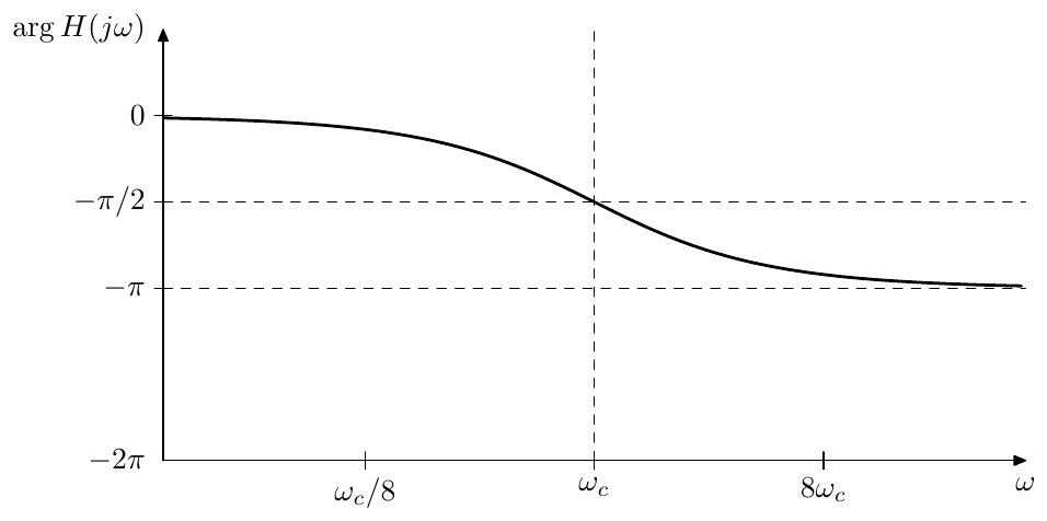
Figure 10.35: Phase response of a 1-pole allpass filter.
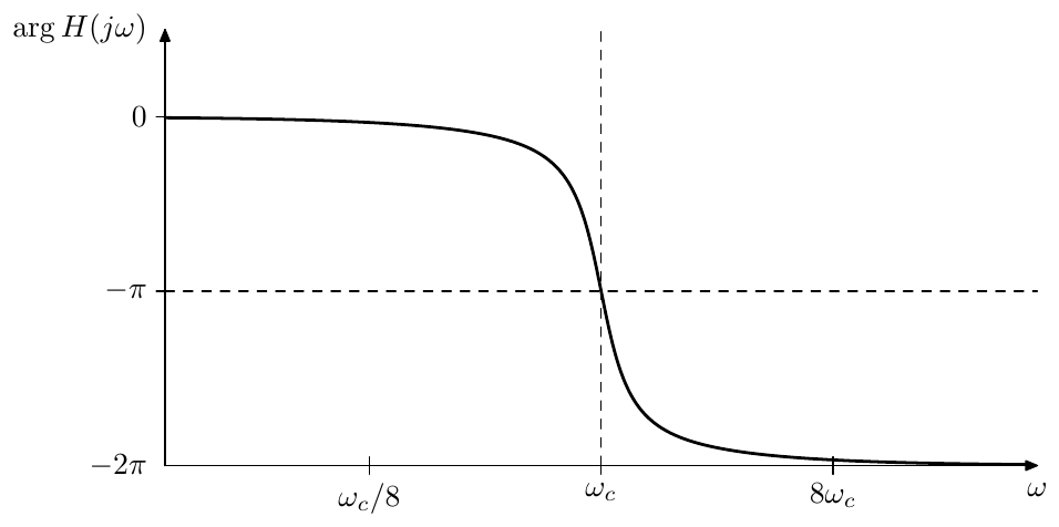
Figure 10.36: Phase response of a 2-pole allpass filter.
Using cutoffs of alternating signs, we rewrite the transfer function expression (10.83) as
(the cutoff of needs to be positive in order for the phase response of to have a negative derivative at ). Considering that the phase response of a 1-pole allpass with cutoff is
the phase response of the serial decomposition (10.84) is
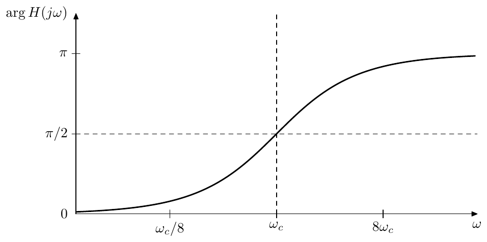
Figure 10.37: Phase response of a negative-cutoff 1-pole allpass filter.
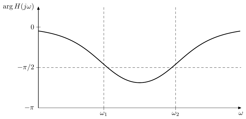
Figure 10.38: Phase response of a pair of a positive-cutoff and a negative-cutoff 1-pole allpass filters. Frequency scale is logarithmic.
where and are the logarithmic scale counterparts of and (essentially these are the pitch-scale values, we have just used rather than 2 as the base to simplify the expressions of the derivatives of ). The reason to use the logarithmic scale in (10.85) is that the phase responses of 1-pole allpasses are symmetric in the logarithmic scale, therefore the entire problem gets certain symmetry and uniformity.
Now we are in a position to specify the minimax approximation problem of construction of the phase shifter . We wish to find the minimax approximation of on the specified interval , where the approximating function needs to be of the form (10.85).
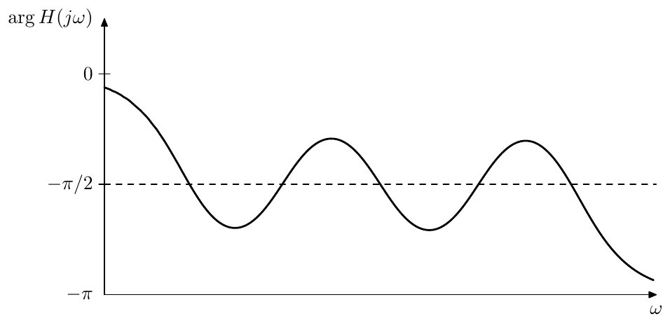
Figure 10.39: Phase response of a series of alternating positive-cutoff and negative-cutoff 1-pole allpass filters. Frequency scale is logarithmic.
The approximating function has parameters:
which can be found by using the Remez algorithm for approximations of general form. Notably, for larger and smaller intervals the problem becomes more and more nonlinear, requiring smaller damping factors in (10.81) and (10.82). The damping factors may be chosen by restricting the lengths and in (10.81) and (10.82).
In order to further employ the logarithmic symmetry of the problem (although this is not a must), we may require corresponding to . Then the following applies.
-
Due to the symmetry the obtained cutoffs will also be symmetric: . (Actually they will be symmetric relatively to no matter what the and are, but it’s convenient to have this symmetry more explicitly visible.)
-
Using this symmetry the number of cutoff parameters can be halved (for odd the middle cutoff is always at unity and therefore can be also excluded from the set of varying parameters). Essentially we simply restrict to be an odd (for odd ) or even (for even ) function of .
-
The obtained symmetric range can be scaled by an arbitrary constant by scaling the allpass cutoffs by the same constant:
Figs. 10.40 and 10.41 contain example approximations of obtained by cutoff optimization (for the demonstration purposes, the approximation orders have been chosen relatively low, giving the phase ripple amplitude of an order of magnitude of ). The readers are encouraged to compare these pictures (qualitatively, since the specified filter orders and bandwidths do not match) to Fig. 10.28.
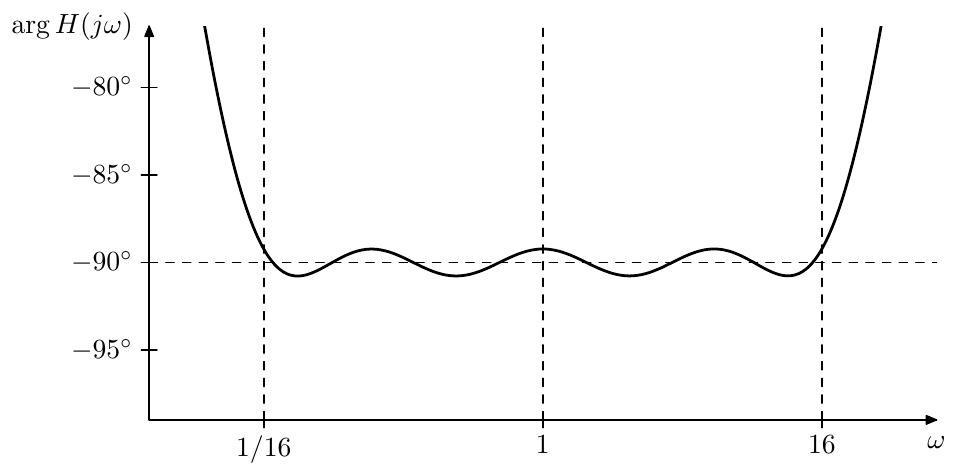
Figure 10.40: 8th-order minimax approximation of the ideal .
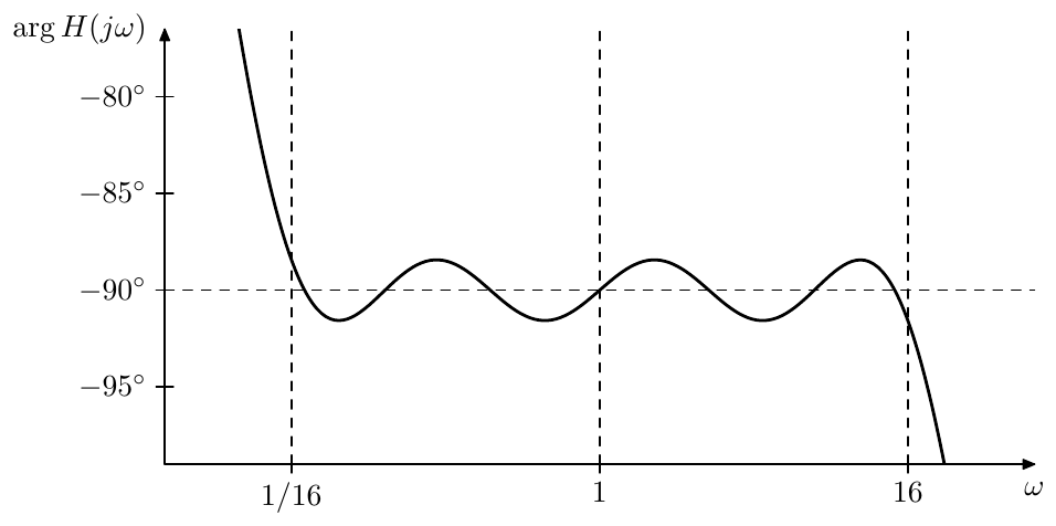
Figure 10.41: 7th-order minimax approximation of the ideal .
Instead of solving the initial approximation equation (10.82) there is a different approach, which generally results in the nonlinearity of not so strongly affecting the algorithm convergence. We could take the manually constructed (10.84) with 4-octave spaced cutoffs as our initial approximation. The formal range of interest could contain two additional octaves on each side: , . Employing the logarithmic symmetry, we center the whole range around , so that .
Using (10.81) (in the logarithmic scale ) we refine the initial approximation to the ripples of equal amplitude. Then we simply shrink the range a little bit. An efficient shrinking substitution is using the geometric averages:
The substitution (10.86) doesn’t affect the control points or the zeros of the Remez algorithm. Therefore after the substitution the Remez algorithm can be simply run again. Then the substitution is performed again, and so on, until we shrink the interval to the exact desired range.34
Notice that the approximations on the intermediate ranges do not need to be obtained with a very high precision, since their only purpose is to provide a starting point for the next application of the Remez algorithm on a smaller range. It is only the Remez algorithm on the exact desired range, which needs to be run to a high precision. This can noticeably improve the algorithm’s running time.
Summary
We have discussed various approaches to the construction of shelving filters, crossovers and Hilbert transformers. The basis for the construction happened to be mostly EMQF filters, with 1st-kind Butterworth as their limiting case. The slope control in higher-order shelving filters was implemented using 2nd-kind Butterworth filters, although EMQF filters can also be used here with the drawback of having ripples in the pass and shelving bands.
Further reading
S.J.Orfanidis, Lecture notes on elliptic filter design (available on the author’s webpage).
M.Kleehammer, Mathematical development of the elliptic filter (available in QSpace online repository).
Elliptic filter (Wikipedia artile).
L.M.Milne-Thomson, Jacobian elliptic functions and theta functions and Elliptic Integrals (contained in Handbook of mathematical functions by M.Abramowitz and I.A.Stegun, available on the internet).
-
Notice that incidentally this implies that is a discrete-time allpass transfer function, although not necessarily describing a stable allpass. ↩
-
The author has learned the approach of constructing a shelving filter as a ratio of two lowpasses from Teemu Voipio. ↩
-
It would have been okay, if all zeros of were at the origin, since in this case the zeros of and would be also at the origin and therefore would cancel each other. Particularly, we could have used Butterworth highpass filters in (10.6), but this wouldn’t have produced any new results compared to Butterworth lowpasses. ↩
-
The other option implied by (10.10) implies , therefore we ignore it. ↩
-
It’s not difficult to realize that the 6 in the denominator is 1-pole lowpass filter’s rolloff of 6dB/oct. ↩
-
This can be derived from the fact that in this case has real poles and zeros which are mutually reciprocal. Thus, each such reciprocal pole/zero pair makes up a 1-pole tilting filter. The gain of the tilting 2-pole filter is distributed into two 1-pole tilting filter’s gains, each equal to . ↩
-
Since the 2-pole tilting filter is essentially a ratio of two 2-pole lowpass filters with mutually reciprocal cutoffs, and since these lowpasses obtain a resonance peak at , it is intuitively clear that either immediately below or possibly starting from a slightly lower boundary these peaks will show up in amplitude response of the tilting filter. In Section 10.7 we will establish that at the filter will go into elliptic range, and it will follow that the elliptic ripples (showing up as resonance peaks for 2nd-order filters) will appear immediately below . ↩
-
Note that the relative steepness of the amplitude response thereby provides a natural way to control the steepness variation, where , where is the actual derivative of the amplitude response at the midpoint and is the same derivative for (for the currently chosen tilting amount ). ↩
-
Unfortunately there is no 100% generalization of this process for lowpass, highpass or bandpass filters, since the rolloff of these filter types is fixed to an integer multiple of 6dB/oct and can’t be varied in a smooth way. ↩
-
Alternatively, by multiplying the response by we obtain a kind of “inverted band-shelving” filter, where the shelving bands are to the left and to the right of the passband in the middle. ↩
-
Thus, differently from how we used (9.152) in the discussion of elliptic lowpass, we treat and now as independent variables. This doesn’t affect the solution process of (9.152), since the respective transformations didn’t use the interdependency of and . ↩
-
We should mind that the dependency between the transition bandwidth and is reciprocal-like: larger means smaller bandwidth. The other two dependencies are straightforward. ↩
-
Particularly, notice that (10.25) becomes identical to (10.17) for . ↩
-
Notice that such switching is completely smooth, as the transfer functions of the filters are completely identical at this point and the “physical” orders of the filters are identical too (there is no pole/zero cancellation as we had in the Butterworth filter order switching). Strictly speaking, the statement that the transfer functions are identical holds only under the restriction that the phase responses of the filters are in sync, rather that off, which is a matter of the sign in front of the transfer functions. However usually we are having zero phase responses at , therefore the signs will be automatically matched. ↩
-
In principle, by general considerations, one should be able to connect two identical parallel representations in series and obtain modal mixtures from those in a fashion similar to the multimode serial cascade. The author however didn’t verify the feasibility of this approach. ↩
-
The author has been made aware of the importance of the in-phase property of Linkwitz- Riley crossovers by a remark by Teemu Voipio. The author also learned the cascaded phase correction approach shown in Fig. 10.24 from the same person. ↩
-
The idea to generalize the Linkwitz-Riley design arose from a remark by Max Mikhailov, that Linkwitz-Riley crossovers can be also built based on naive 1-pole lowpasses, which in the BLT terms can be formally seen as a special kind of high-shelving filters. It is quite possible that this idea has been already developed elsewhere, however at the time of the writing the author is not aware of other sources. ↩
-
In order to show that this factoring is possible, multiply by , obtaining , where the latter inequality follows from . ↩
-
This would have been formally possible if is allowed to be unstable, however the order of would have been equal to the sum of the orders of and . We mention this because this has a clear analogy to the phase splitter discussed later in the text. ↩
-
The identity transfer function 1 in the left-hand side obviously has no poles, but we could also write it as in which case it formally has the same poles (which are then cancelled by the zeros). ↩
-
Since we want our allpass approximation of to be a real filter, its phase response must be odd, which leaves only two possible values at : or . If we formally include into the range of frequencies of interest, then we notice that the phase response at has the same two options. ↩
-
In order to convince oneself that this is indeed so, one could factor a generic stable allpass tranfer function into 1st- and 2nd-order sections and consider their phase responses, which are monotonically decaying. ↩
-
Except that we would obtain both stable and unstable poles this time, since there is no explicit restriction of the solutions having to be in the left semiplane. ↩
-
Apparently the imaginary axis belongs to the family of lines shown in Fig. 9.54, being the boundary case between the two groups of lines on the left and on the right. ↩
-
The same reasoning can be applied to (10.45), where we want the imaginary signal to be phase shifted by compared to the real one. Therefore the lowest-cutoff allpass factor (corresponding to the pole closest to the origin) must be in the imaginary signal’s allpass. Since the poles of the allpasses in (10.45) are obtained by Riemann sphere rotation , the pole closest to the origin will be obtained from the pole closest to , which is an even pole for odd and an odd pole for even. ↩
-
Note that if desired, we can also find from by (9.110) (where we let ). ↩
-
The signal notations and denote the positive- and negative-shifted signals respectively and shouldn’t be confused with the “+” and “-” subscripts of and which denote the stable and unstable poles. ↩
-
The description of Remez algorithm (which is a numerical minimax optimization algorithm) was included into earlier revisions of this book as an alternative to the use of elliptic functions to construct phase splitters. Now that the book is strongly focusing on elliptic functions anyway, the discussion of Remez algorithm might feel almost redundant. However the author felt that this is still quite valuable resource to be simply dropped from the book. Particularly, Remez algorithm is useful for building low-cost approximations of functions, although, depending on the context, minimax solutions are not necessarily the best ones for a given purpose. ↩
-
The maximum of the absolute value of a function is also the norm of the function. Therefore minimax approximations are optimizations of the norm. ↩
-
The Remez algorithm should not be confused with the Parks-McClellan algorithm. The latter is a specific restricted version of the former. For whatever reason, the Parks-McClellan algorithm is often referred to as the Remez algorithm in the signal processing literature. ↩
-
The author’s primary resource for the information about the Remez algorithm was the documentation for the math toolkit of the boost library by J.Maddock, P.A.Bristow, H.Holin and X.Zhang. ↩
-
This becomes kind of intuitive after considering Chebyshev polynomials as some kind of minimax approximations of the zero constant function on the interval . ↩
-
This trick is adapted from the boost library documentation and sources. ↩
-
Of course at the last step we simply set and to the desired values, rather than perform the substitution (10.86). ↩