Chapter 8: Raising the filter order
As the order of the filter grows, there are more and more different choices of the transfer function. Particularly, there is more than one way to introduce the resonance into a transfer function of order higher than 2. Some of the most interesting options were already discussed in the previous chapters.
We have also introduced the state-space form as a general representation for differential systems. However, being so general, the state-space form leaves lots of open questions in regards to the choice of topology and the user-facing parameters.
In this chapter we are going to discuss a number of standard topologies which can be used to construct a system of any given order and also a number of ways to map commonly used user-facing parameters, such as cutoff and resonsance, to the internal parameters of such systems. Note, however, that these structures and techniques are useful only occasionally, for rather specific purposes.
8.1 Generalized SVF
We have seen that the idea of the ladder filter can be generalized from a 4-pole to other numbers of poles, even though there are problems arising at pole counts other than 4. Could we somehow attempt to generalize the SVF?
The most natural way to generalize the SVF is probably to treat it as the so-called controllable canonical form, (Fig. 8.1) which is the analog counterpart of direct form II (Fig. 3.33). Apparently, the main difference between Fig. 3.33 and Fig. 8.1 is simply that all unit delays are replaced by integrators. The other differerence, namely the inverted feedback is merely a matter of convention, resulting in opposite signs of the coefficients compared to what they would have been in the absence of the feedback inversion. We chose the convention with the inverted feedback mainly because it’s more similar to the 2-pole SVF structure in Fig. 4.1.
The controllable canonical form allows to implement an arbitrary transfer function of -th order (the requirement that the transfer function is a non-strictly proper rational function being implicitly understood). Indeed, it’s not difficult to figure out that the tranfer function of the system in Fig. 8.1 is
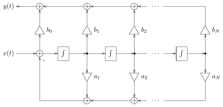
Figure 8.1: Generalized SVF (controllable canonical form).
Thus and are simply the denominator and numerator coefficients of the transfer function. Notice that are essentially modal pickups and we can share the feedback part of the structure (consisting of integrators and gains) among several different sets of pickup coefficients to simultaneously implement a number of filters sharing a common denominator.
Normally Fig. 8.1 assumes unit-cutoff integrators, because the and coefficients provide enough freedom to implement any transfer function of the given order. However, in music DSP applications cutoff control is a common feature, therefore we could also allow the integrators to take identical non-unit cutoffs. Further, letting , and we obtain an SVF with serving as modal mixing coefficients for HP, BP and LP outputs. On the other hand, at , we obtain the 1-pole filter we discussed in the beginning of this book.
Generally, letting have a fixed value is a good way to remove the redundancy introduced into the system control by the embedded cutoffs of the integrators. It is not difficult to realize that
where are the positions of the system poles when . Notably, although it is mostly academic, this also can support the case of real poles of opposite signs, which cannot be implemented by a classical 2-pole SVF due to being fixed to 1.
Unfortunately, there is no clear answer to what the coefficients should be for . The simplicity of the 2-pole case was due to the fact that the denominator of a 2-pole transfer function essentially has only 2 degrees of freedom (corresponding to and ), one degree being taken by the cutoff, and we are being left with the remaining degree which just happens to correspond to the resonance. With the 1-pole there was only one freedom degree, being taken by the cutoff. At there are too many different options of how to map the freedom degrees to filter control parameters and there is no definite answer to that, although some of the options will be discussed later in this chapter.
With the numerator coefficients there is a bit more clarity, as there are certain general considerations applying more or less for any choice of . E.g. if the numerator is equal to , we get some kind of an -th order lowpass, since and for . For the numerator we have and for , corresponding to some kind of an -th order highpass. For an even and an numerator we get for and for , corresponding to some kind of a bandpass. This however defines only the asymptotic behavior at 0 and , the amplitude response shape in the middle can be pretty much arbitrary, being defined by the denominator.
By transposing the controllable canonical form one obtains the so-called observable canonical form. We are not going to address it in detail, as most of the discussion of the controllable canonical form above applies to the observable canonical form as well.
8.2 Serial cascade representation
Another structure which allows implementing arbitrary transfer functions is the serial cascade. It is probably the one most commonly used. Compared to the generalized SVF, in the serial cascade representation we are using only 1- and 2-pole filters and we can choose commonly known and well-studied structures to implement those.1 The benefit compared to the parallel implementation (discussed later in this chapter) is that the serial cascade form doesn’t get ill-conditioned when system poles get close to each other.
Cascade decomposition
Given an arbitrary -th order real transfer function, let’s write it in the multiplicative form:
where , since must be nonstrictly proper. Since has real coefficients, all complex poles of will come in conjugate pairs, and the same can be said about the zeros.
Now we are going to write each pair of conjugate poles as a purely real 2nd-order factor in the denominator:
and we are going to write each pair of conjugate zeros as a purely real 2nd-order factor in the numerator:
Further, if necessary, we can combine any two real poles into a 2nd-order factor in the denominator:
and we can combine any two real zeros into a 2nd-order factor in the numerator:
Thus we can distribute all conjugate pair of poles and zeros into 2nd-order real rational factors of the form
unless we do not have enough zeros, in which case there will be one or more 2nd-order real rational factors of the form
The remaining pairs of real poles and zeros can be combined into 1st-order real rational factors of the form
or they can be also combined into 2nd-order real rational factors, e.g.:
Thus the entire transfer function is represented as a product of purely real 2nd- and 1st-order factors:
where and are the 2nd- and 1st-order factors respectively. The gain coefficient , if desired, can be factored into the numerator of one or several of the factors and , so that the product expression gets a simpler form:
Now recall that 1-pole multimode can implement any stable real 1st-order transfer function and SVF can implement any stable real 2nd-order transfer function. This means that we can implement pretty much any as a serial chain of SVFs2 and 1st-order multimodes.3 We will refer to the process of representing is a cascade form as cascade decomposition of .
Cutoff control
The denominator of a 1-pole filter is controlled by a single parameter, which is the filter cutoff. The denominator of a 2-pole filter is controlled by cutoff and damping. Thus each of the 2- and 1-poles in (8.3) has a cutoff, defined by the positions of the respective poles. Writing explicitly these cutoff parameters in (8.3) we obtain
where and are unit-cutoff versions of the same 2- and 1-poles and and are the respective cutoffs.
Suppose the above defines a unit-cutoff filter. Then non-unit cutoff for is achieved by
which means that the cutoffs of the underlying 2- and 1-poles are simply multiplied by and we have and as the 2- and 1-pole cutoffs.
One should remember, that it is important to apply one and the same prewarping for all filters in the cascade, as discussed in Section 3.8. E.g. we could choose to prewarp (8.4) at , which means that we prewarp only (rather than individually prewarping the 2- and 1-pole cutoffs and ), thereby obtaining its prewarped version , and then simply substitute for in (8.4):
Thus, the 2- and 1-pole cutoffs become and respectively.
Cascaded model of a ladder filter
As an example of the just introduced technique we are going to implement the transfer function of a 4-pole lowpass ladder filter by a serial chain of two SVFs. A 4-pole lowpass ladder filter has no zeros and two conjugate pairs of poles for . By considering two coinciding poles on a real axis also as mutually conjugate, we can assume .
Since there are no zeros, we simply need a 2-pole lowpass SVF for each conjugate pair of poles. Let , , , be the poles of the ladder filter. According to (5.2)
By (4.13), the cutoffs of the 2-pole lowpasses and . Respectively the transfer function of the ladder filter can be represented as
The unknown gain coefficient can be found by evaluating (5.1) at , obtaining the condition . Evaluating (8.6) at yields . Therefore
This gives us a cascade of 2-poles implementing a unit-cutoff ladder filter. Extending (8.6) to arbitrary cutoffs is respectively done by
Cascaded multimode
The cascade decomposition can be also used to provide modal outputs, sharing the same transfer function denominator. In order to demonstrate this we will consider a serial connection of two SVFs.4
The transfer function of such structure can have almost any desired 4th order stable denominator.5 We would like to construct modal outputs for such connection, so that by mixing those modal signals we should be able to obtain arbitrary numerators. This should allow us to share this chain of SVFs for generation of two or more signals which share the same transfer function’s denominator.
We have several options of connecting two SVFs in series, depending on which of the modal outputs of the first SVF is connected to the second SVF’s input. The most symmetric option seems to be picking up the bandpass output (Fig. 8.2).
Now let
be the denominators of the transfer functions of the two SVFs and let be their product. Writing out the transfer functions for the signals at the SVF outputs (in respect to the input signal in Fig. 8.2) we obtain
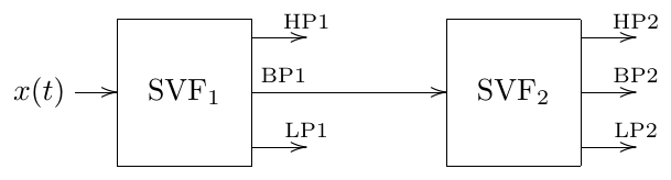
Figure 8.2: A multimode cascade of two SVFs.
Or, since we have the common denominator everywhere, we could concentrate just on the numerators:
Noticing from Fig. 8.2 that BP1 can be obtained as LP2 + BP2 + HP2 anyway, we can drop the respective numerator from the list and try to arrange the remaining ones in the order of the descending polynomial order:
The last line doesn’t really fit, and the first one looks more complicated than the next three, but we can fix that by replacing the first and the last lines by linear combinations:
Thus we can obtain all powers of from linear combinations of LP1, HP1, LP2, BP2 and HP2, thereby being able to construct arbitrary polynomials of orders up to 4 for the numerator.
Notably, instead of connecting the bandpass output of the first SVF to the input of the second SVF, as it has been shown in Fig. 8.2, we could have connected the lowpass or the highpass output. This would have resulted in somewhat different math, but essentially gives the same modal mixture options.
8.3 Parallel representation
Real poles
Given a transfer function which has only real poles which are all distinct, we could expand it into a sum of 1st-order partial fractions. Each such 1st-order fraction corresponds to a 1-pole and we could implement the transfer function as a sum of 1-poles. Essentially this is identical to the diagonal state-space form, which, provided all system poles are real and sufficiently distinct (so that no ill-conditioning occurs), is just a set of parallel Jordan 1-poles.
In the case of a single-input single-output system, which we are currently considering, the transfer function of such diagonal system, given by (7.18), has the form
where and are the input and output gains respectively. Given a particular nonstrictly rational , the partial fraction expansion (8.7) uniquely defines and the products . The respective freedom of choice of and can be resolved by letting and thus we control the numerator of the transfer function by the output mixing coefficients (Fig. 8.3).6
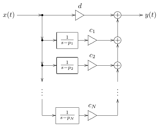
Figure 8.3: Implementation by parallel Jordan 1-poles.
We could also replace Jordan 1-poles by ordinary 1-pole lowpasses, where we need to divide the mixing coefficients by the respective cutoffs (Fig. 8.4).
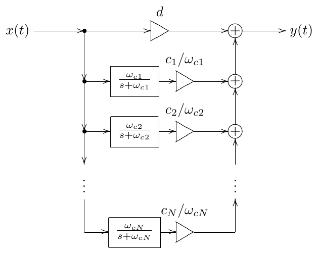
Figure 8.4: Implementation by parallel 1-pole lowpasses.
The global cutoff control of the entire filter in Fig. 8.3 or Fig. 8.4 is achieved in the same way as with serial cascades. Obviously, the usual consideration of common prewarping of the 1-pole components applies here as well.
Complex poles
If system poles are complex we need to use the real diagonal form, which replaces the complex Jordan 1-poles with Jordan 2-poles. For a single-input single- output system, equation (7.28) takes the form
We could obtain the explicit expressions for and from the derivation of (7.28), but it would be more practical to simply obtain their values from the partial fraction expansion of . That is, given , we find and (as well as, of course, and ) from (8.8). We also should remember that, according to the freedom of choice of the state space basis vectors lengths, we could choose any non-zero input gains vector, e.g. which means that we are using only the “real part” input of the Jordan 2-pole.7 According to (7.26), the contribution of such Jordan 2-pole to will be
Thus
from where
Thus, having found and , we can find and . The respective structure is shown in Fig. 8.5. Notice that as becomes smaller, becomes larger. This is the ill-conditioning effect of the diagonal form discussed in Section 7.11.
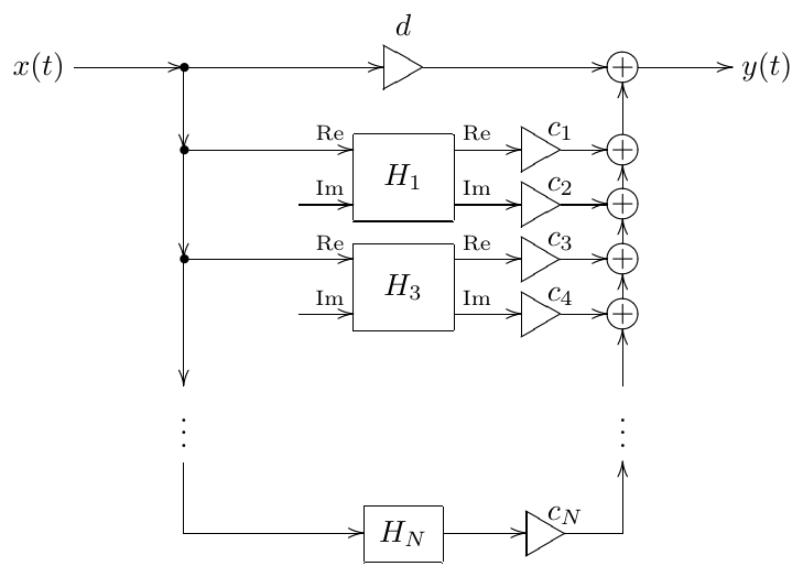
Figure 8.5: Implementation by parallel Jordan 2- and 1-poles. Disconnected imaginary part inputs are receiving zero signals.
Similarly to how we could replace Jordan 1-poles with ordinary 1-pole lowpasses, we could replace Jordan 2-poles by some other 2-poles, e.g. by SVFs. Finding the output mixing coefficients becomes simpler, since, apparently, the coefficients and in (8.8) now simply correspond to SVF bandpass and lowpass output gains (properly scaled by the cutoff). Fig. 8.6 illustrates.
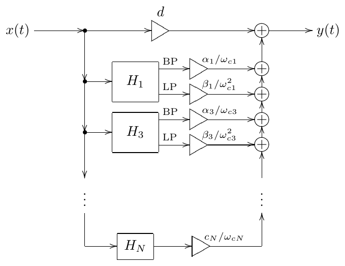
Figure 8.6: Implementation by parallel SVFs and 1-pole lowpasses.
Another benefit of an SVF is that it doesn’t have a problem at the point where its poles coincide and also can support the case of real poles, meaning that we could convert arbitrary pairs of parallel 1-poles into an SVF. The same apparently could be done by an SKF/TSK. There would still be a problem though, if poles of different parallel 2-poles coincide, resulting in the already known ill-conditioning effect.
Regarding the cutoff control of the entire system, there is no difference from the parallel 1-poles case.
Coinciding poles
Generally, anything with repeated or close to each other poles cannot be implemented in a parallel form and needs some non-parallel implementation (SVF, a chain of SVFs, Jordan chain, etc.) However the implementation could still be partially parallel, where the poles may be repeated within each block, but different parallel blocks shouldn’t have poles at the same locations.
8.4 Cascading of identical filters
So we have learned a number of different ways to implement higher-order transfer functions, of which cascaded form is said to be usually the best option, however, how do we construct these transfer functions in the first place? E.g. how do we generalize a resonating 2-pole transfer function to a 4-th or 8-th order? Or how do we generalize a 1-st order lowpass to a 5-th or 8-th order?
One possible way which could immediately occur to us is to stack several identical filters together. Note that, given a filter with the transfer function and another one with the transfer function and looking at their decibel-scale amplitude responses, we notice that the latter is simply the former multiplied by , that is the amplitude response becomes scaled times vertically (obviously, the same scaling is happening to the phase response). Particularly this means that the rolloff slope of the filter becomes times steeper.
Therefore in order to generalize a 1-st order lowpass to the -th order we could simply connect such lowpasses in series:
resulting in the amplitude response curve in Fig. 8.7. It looks as if the cutoff of is is too low. In principle we could address this by shifting the filter cutoff, so that . In order to do so we solve the equation
obtaining the frequency which should be treated as the cutoff point of each of the chain’s elements:
so the transfer function becomes
This looks a bit better (Fig. 8.8) and can be taken as a possible option.
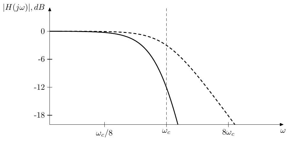
Figure 8.7: Amplitude response of a 1-pole lowpass filter (dashed) vs. amplitude response of a serial chain of 4 identical 1-pole lowpass filters (solid).
In the same way we could generalize a resonating 2-nd order lowpass to the -th order by connecting of such lowpasses together
However in this case the situation is somewhat worse than with 1-poles. First we notice that the resonance peak becomes much higher at the same damping (Fig. 8.9). At first sight it doesn’t look like a big problem, we could simply use smaller values of the damping. However if we compare the amplitude response curves of a 2-pole vs. stacked 2-poles with the damping adjusted to produce the same peak height,8 we notice that due to the now smaller damping value the resonance peak of the 2-pole chain is much wider than the peak of a single 2-pole (Fig. 8.10), all in all not a very desirable scenario.
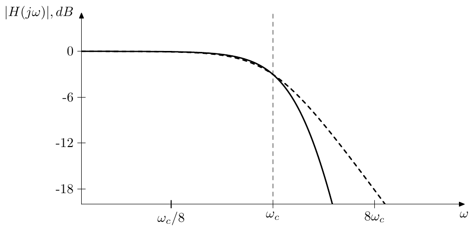
Figure 8.8: Amplitude response of a 1-pole lowpass filter (dashed) vs. amplitude response of a serial chain of 4 identical 1-pole lowpass filters with adjusted cutoff (solid).
8.5 Butterworth transformation
We have seen that cascading identical filters is one possible way to obtain higher-order filters, which effectively scales the decibel-scale amplitude response and the phase response of the filter times vertically, respectively making the filter rolloff times steeper.
Another way to make the rolloff times steeper would be finding a transformation which shrinks the amplitude response in the logarithmic frequency scale times:
(where we don’t care about because for real filters , and where ). Or equivalently
The readers may recall the LP to HP transformation which flips the responses in the logarithmic frequency axis. One could try to draw an analogy and attempt substitutions of the form or (, ), however it’s not difficult to convince oneself that such substitutions do not work. Nevertheless, the basic direction is mostly right. Just instead of of performing an argument substitution on the transfer function, we will directly apply (8.10) to the amplitude response . That is we will be looking for such that
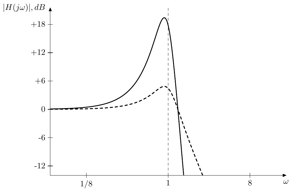
Figure 8.9: Amplitude response of a 2-pole filter (dashed) vs. amplitude response of a serial chain of 4 identical 2-pole filters (solid).
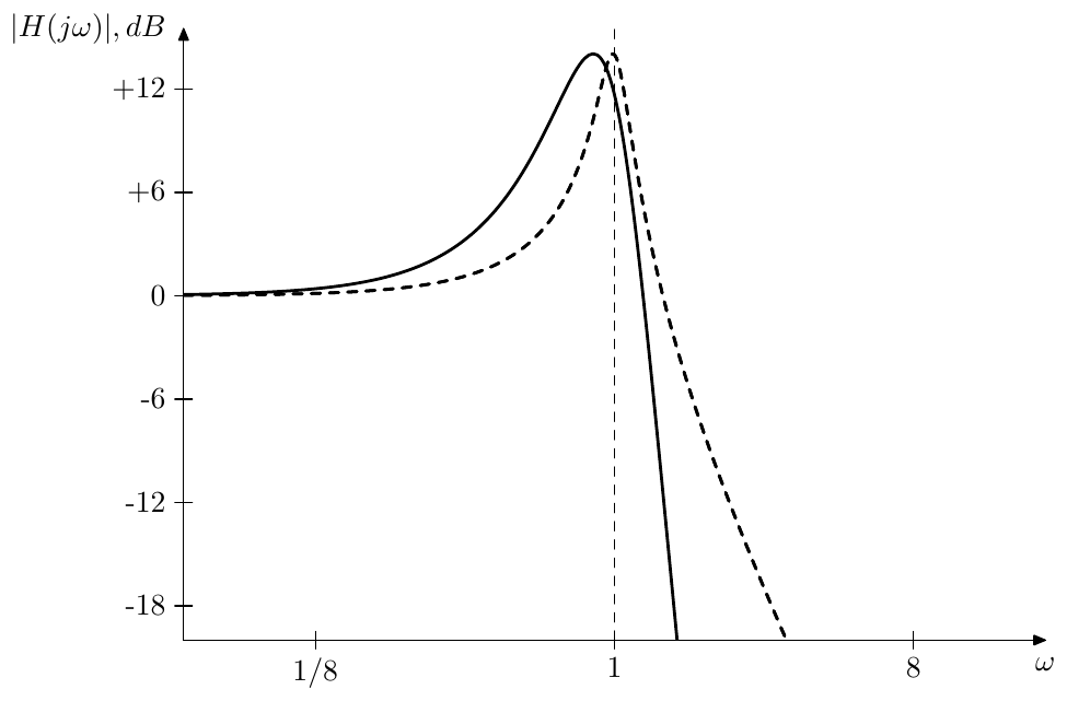
Figure 8.10: Amplitude response of a 2-pole filter (dashed) vs. amplitude response of a serial chain of 4 identical 2-pole filters with adjusted damping (solid).
We will refer to the transformation of into defined by (8.11) as Butterworth transformation.9 The integer will be respectively referred to as the order of the Butterworth transformation. We will denote Butterworth transformation as
or, if we want to explicitly specify the order
where denotes the new transfer function obtained as the result of the transformation.10
Without having developed the transformation details yet, we can already establish several properties of this transformation, which follow from (8.11):
- the transformation doesn’t change a constant function:
- a constant gain can be simply factored out of the transformation:
- a change of the cutoff is shrunk times in the logarithmic scale after the transformation:
- the transformation commutes with LP to HP substitution
- the transformation distributes over multiplication:
- the transformation distributes over division:
- Butterworth transformations can be chained:
Since (8.11) doesn’t uniquely define the transformation result, the above properties have to be understood in the sense that the right-hand side can be taken as one possible result of the transformation in the left-hand side. However the amplitude responses of the transformation results are uniquely defined and in those terms the above properties can be understood as usual equalities. E.g. the property (8.12g) can be understood as
Instead of developing Butterworth transformation immediately for arbitrary order filters we are going to first find a way to apply it to 1-pole filters and then to 2-pole filters. At that point we will be able to simply use the property (8.12e) to apply Butterworth transformation to arbitrary-order filters by representing these arbitrary order filters as cascades of 1-st and 2-nd order filters.
8.6 Butterworth filters of the 1st kind
As we just mentioned, first we will develop a way to apply Butterworth transformation to 1-pole filters, in which case we will more specifically refer to this transformation as Butterworth transformation of the 1st kind. The results of Butterworth transformation of the 1st kind coincide with filters commonly known as Butterworth filters. However in this book later we will generalize the idea of Butterworth filters to include the results of Butterworth transformation of filters of orders higher than 1. In order to be able to tell between different kinds of Butterworth filters, we are going to more specifically refer to the filters obtained by Butterworth transformation of 1-pole filters as Butterworth filters of the 1st kind.
Considering that a 1-pole transfer function is essentially a ratio of two 1st-order polynomials
and that the amplitude response of can be written as a ratio of formal amplitude responses of these polynomials:
it is sufficient to develop the transformation for 1st-order polynomials. The transformation of can be then trivially obtained as:
where and are transformed polynomials and .
Transformation of polynomial
We begin by obtaining the Butterworth transformation of the polynomial . Its formal amplitude response is
and we wish to find such that
In order to get rid of the square root we can deal with squared amplitude response instead
Now we would like to somehow obtain from the latter equation.
In order to do so, let’s notice that
where , so the roots of consist of the root of at and of its origin-symmetric image at , the latter being the root of . This motivates to introduce such that
and then try to factor it into in such a way that
In order to find the possible ways to factor into let us find the roots of . Instead of solving for let’s solve for , where we formally let take complex values. The solutions in terms of are related to the solutions in terms of through .
Solving for we obtain
The solutions are illustrated in Figs. 8.11 and 8.12 where the complex plane can be alternatively interpreted in terms of or in terms of (note the labelling of the axes), thus these figures simultaneously illustrate the solutions in terms of or in terms of . Thus the roots of are equally spaced on a unit circle with an angular step of . If is odd there will be roots at otherwise there are no real roots.
Another possible way to look at the solutions of is to rewrite the equation as
In this case the roots obtained from the equation will be interleaved with the roots obtained from the equation (Figs. 8.11 and 8.12 illustrate). Sometimes therefore such roots are referred to as even and odd roots respectively, since they occur respectively at even and odd in (8.13). This distinction usually can be ignored, but occasionally becomes important.
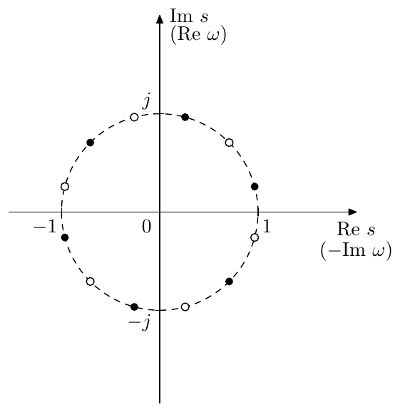
Figure 8.11: Roots of for the Butterworth transformation of the 1st kind of an even order (). White and black dots correspond to even and odd roots.
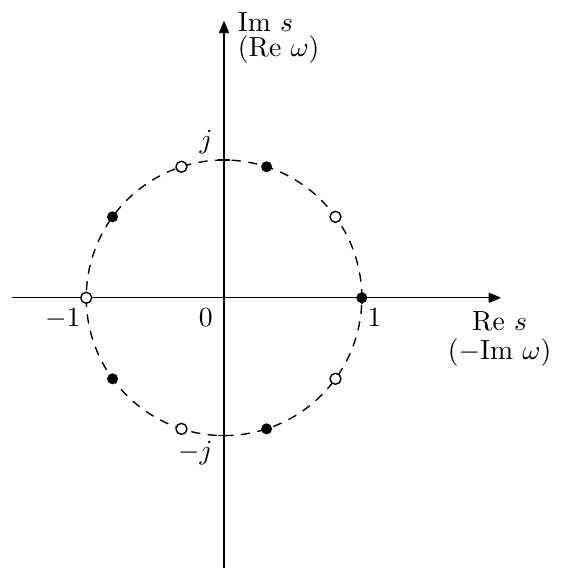
Figure 8.12: Roots of for the Butterworth transformation of the 1st kind of an odd order (). White and black dots correspond to even and odd roots.
Having found the roots of how do we split them into the roots of and the roots of ? Obviously we cannot do this splitting in an arbitrary way, since there are several special properties which need to be satisfied.
-
For any possible polynomial its roots are origin-symmetric to the roots of , so our root splitting must respect this property.
-
must be a real polynomial. This requires its roots to be either real or coming in complex conjugate pairs.
-
If is the denominator of the filter’s transfer function, then its roots must be located in the left complex semiplane (in order for the filter to be stable).
-
The requrement implies . In order to satisfy the latter, the roots of must be symmetric to the roots of with respect to the imaginary axis (essentially it is the same reasoning which we had in the discussion of minimum phase and maximum phase zero positioning).
Looking at Figs. 8.11 and 8.12 it’s not difficult to notice that all of the above requirements will be satisfied if we choose the roots in the left complex semiplane to be the roots of and the roots in the right complex semiplane as the roots of respectively.11
Having found the roots of we still need to find the leading coefficient of :
In order to do so, notice that (8.11) implies . Since and we should have . Actually, if we let we will obtain . Indeed,
That is is equal to the product of all roots of . Looking at Figs. 8.11 and 8.12 we notice that the product of all roots of is equal to 1 and thus .12
Thus, by finding the roots and the leading coefficient of we have obtained a real polynomial in the multiplicative form. In practical filter implementations the complex conjugate pairs of factors of will be represented by 2nd-order filter sections, the purely real factor of appearing for odd will be represented by a 1st-order filter section:
where
stands for bitwise conjunction.
Arbitrary 1st-order polynomials
Considering of a more generic form () we notice that essentially the procedure is the same as for except that instead of the equation we obtain the equation
This means that the roots of are no longer located on the unit circle but on a circle of radius . It is not difficult to see that the leading coefficient of is still equal to 1.
The above result also could have been obtained by rewriting as and applying properties (8.12b) and (8.12c), which on one hand gives a more intuitive understanding of why the circle of roots is scaled by , on the other hand can serve as an explicit proof of (8.12c) for the case of Butterworth transformation of the 1st kind.
The case of () can be obtained as a limiting case13 resulting in .
If then, noticing that the amplitude responses of and are identical (for ), we could obtain as Butterworth transformation of . However, since the root of is in the right semiplane, it would be logical to also pick the right semiplane roots of as the roots of . Particularly, if is the numerator of a maximum phase filter, the transformation result will retain the maximum phase property.
The 1st-order polynomials of the most general form can be treated by rewriting them as , if . The case of can be simply treated as a limiting case , where we drop the vanishing higher-order terms of , resulting in .
Lowpass Butterworth filter of the 1st kind
Given
we transform the denominator according to the previous discussion of the Butterworth transformation of a 1st order polynomial. The roots of the transformed polynomial (located on the unit circle) become the poles of . The numerator of is obviously unchanged by the transformation. Thus we obtain
where the term occurs in case of an odd (“” standing for bitwise conjunction). Therefore can be implemented as a series of 1-pole and 2-pole lowpass filters, where the 1-pole appears in case of an odd .
Fig. 8.13 compares the amplitude response of a Butterworth lowpass filter of the 1st kind () against the prototype 1-pole lowpass filter. One can observe the increased steepness of the cutoff slope resulting from the shrinking along the logarithmic frequency axis. Fig. 8.14 compares the same Butterworth lowpass filter against cascading of identical 1st order lowpasses, that is comparing the shrinking along the logarithmic frequency axis vs. stretching along the logarithmic amplitude axis. One can see that the Butterworth lowpass filter has the sharpest cutoff corner among different filters in Figs. 8.13 and 8.14.
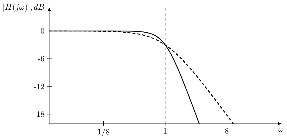
Figure 8.13: 2nd order lowpass Butterworth filter of the 1st kind (solid line) vs. 1st order lowpass filter (dashed line).
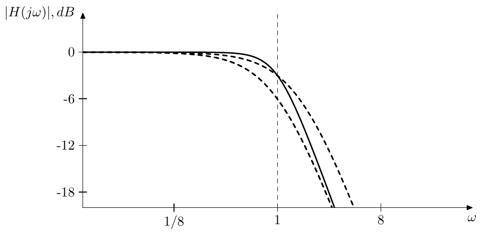
Figure 8.14: 2nd order lowpass Butterworth filter of the 1st kind (solid line) vs. duplicated 1st order lowpass filter without and with cutoff adjustment (dashed lines).
It is useful to know and recognize the expression for the squared amplitude response of a Butterworth lowpass filter of the 1st kind. Since the squared amplitude response of (8.14) is
after the substitution we obtain
This expression is used in traditional derivation of Butterworth filters. Essentially the -th order lowpass Butterworth filter is traditionally defined as a filter whose the amplitude response satisfies (8.15). Note that by (8.15) the 1-pole lowpass is the Butterworth filter of order 1. We can formally treat it as a 1st-order Butterworth transformation of itself
It is also useful to explicitly know the transfer function of the Butterworth lowpass filter of the 1st kind of order . It’s not difficult to realize that for the roots of are located away from the negative real semiaxis. Thus the respective damping is and
This damping value and the 2nd-order term appears in all Butterworth filters of the 1st kind of order (highpass, bandpass, etc.) The readers may also recall the appearance of the damping value in the discussion of 2-pole filters, where it was mentioned that at the 2-pole filter turns into a Butterworth filter. This also corresponds to the fact that among all non-resonating (in the sense of the missing resonance peak) 2nd-order filters the Butterworth filter is the one with the sharpest possible cutoff corner in the amplitude response.
Highpass Butterworth filter of the 1st kind
For
we have the same denominator as for the respective lowpass. Thus the result of the denominator transformation is the same as for the lowpass. The result of the numerator transformation is and thus
That is we obtain the same result as for the 1-pole lowpass, except that instead of a series of lowpasses we should take a series of highpasses. Fig. 8.15 illustrates the respective amplitude response.
It is not difficult to verify that the highpass Butterworth filter obtained in the described above way is identical to the result of LP to HP substitution applied to the lowpass Butterworth filter of the same order, which is in agreement with (8.12d).
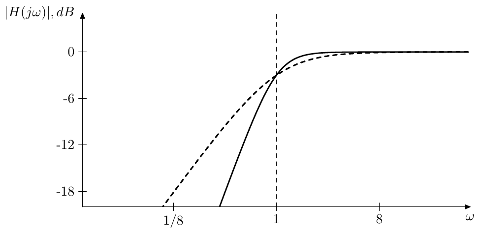
Figure 8.15: 2nd order highpass Butterworth filter of the 1st kind vs. 1st order highpass filter (dashed line).
Bandpass Butterworth filter of the 1st kind
For an even , by formally putting a numerator over the Butterworth transformation of a polynomial we obtain a kind of a bandpass filter:
(Fig. 8.16), which can be also formally seen as a Butterworth transformation of .
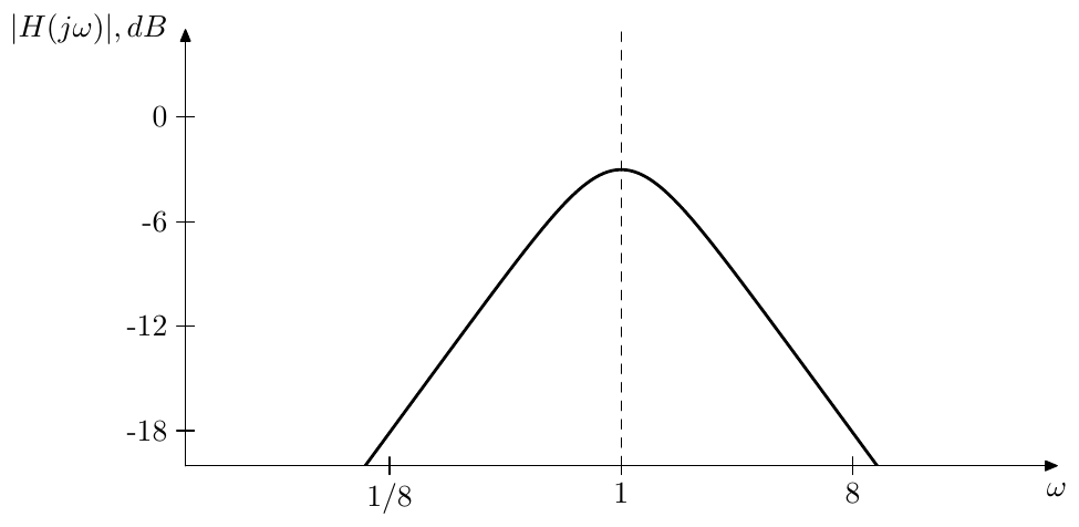
Figure 8.16: 2nd order bandpass Butterworth filter of the 1st kind.
Note that thereby this bandpass filter doesn’t have any parameters to control, except the cutoff. As we will see a bit later in the discussion of Butterworth filters of the 2nd kind, this filter also can be obtained by an order Butterworth transformation of the 2-pole bandpass . Therefore there is not much point in specifically using Butterworth bandpass filters of the 1st kind, one can simply use Butterworth bandpass filters of the 2nd kind instead, achieving exactly the same response at a particular resonance setting.
A bandpass filter which has controllable bandwidth can be obtained by applying the LP to BP substitution to a Butterworth lowpass filter of the 1st kind. Apparently this produces a normalized bandpass (Fig. 8.17). This filter does not coincide with the result of the Butterworth transformation of the normalized 2-pole bandpass . The reason is that in the first case we have a Butterworth transformation of a 1-pole lowpass followed by the LP to BP substitution, while in the second case we first have the LP to BP substitution (with an appropriately chosen bandwidth) applied to yielding , which is then followed by the Butterworth transformation. So it’s the opposite order of the application of LP to BP substitution and the Butterworth transformation.
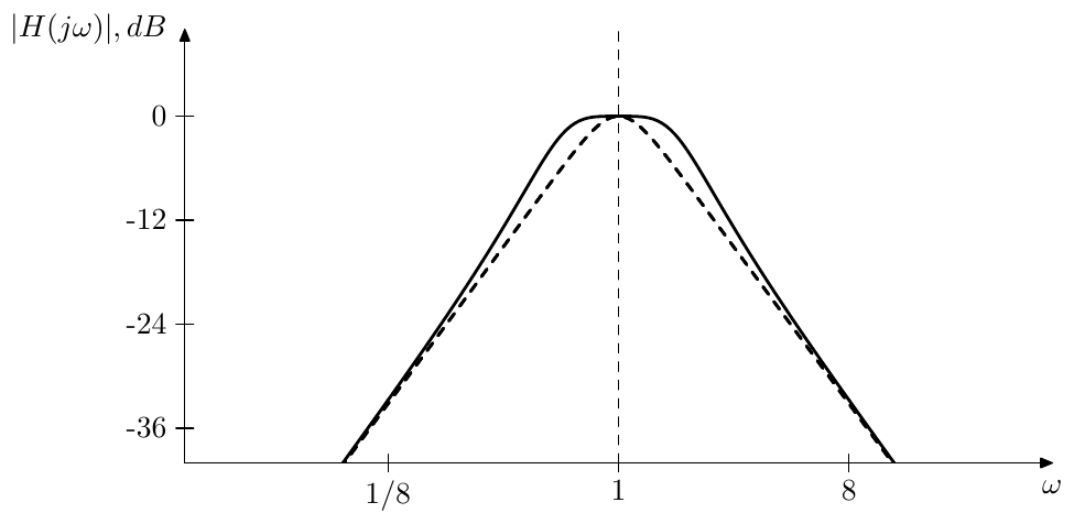
Figure 8.17: A bandwidth-tuned LP to BP substitution of a lowpass Butterworth filter of the 1st kind vs. Butterworth transformation of (dashed line).
The LP to BP substitution can be performed algebraically on the transfer function of the Butterworth lowpass. In order to simplify things, the substitution can be applied in turn to the poles of each of the underlying 1- and 2-pole filters of the cascaded implementation of the Butterworth lowpass. After organizing the transformed poles into mutually conjugate pairs, we can simply construct the result as a series of normalized 2nd order bandpasses, defined by those pole pairs. Alternatively the LP to BP substitution can be implemented using the integrator substitution technique (Fig. 4.19).
8.7 Butterworth filters of the 2nd kind
Now we are going to apply the Butterworth transformation to 2nd order polynomials and respectively 2nd order filters. Such transformation will be referred to as Butterworth transformation of the 2nd kind and the filters obtained as the results of the tranformation will be referred to Butterworth filters of the 2nd kind.
Transformation of polynomial
We will first consider the following 2nd order polynomial
corresponding to the denominator of a unit-cutoff 2-pole filter.
It will be most illustrative to obtain the Butterworth transformation of the 2nd kind as a combination of two opposite perturbations of two Butterworth transformations of the 1st kind. Factoring we obtain
At we have and is a product of two 1st-order polynomials . Applying the Butterworth transformation of the 1st kind to each of the polynomials and we obtain two identical sets of the roots of and respectively. We can also consider the respective (also identical) extended polynomials
which additionally contain the right-semiplane roots. As we should remember from the discussion of the Butterworth transformation of the 1st kind, the roots in each of the two sets corresponding to and are equally spaced on the unit circle.14
Now suppose we initially have and then increase to a value , resulting in growing and decreasing, staying reciprocal to each other:
(Fig. 8.18). Since and are the “cutoffs” of the 1st-order polynomials and , from the properties of the Butterworth transformation of the 1st kind we obtain that the radii of the circles, on which the roots of and are located, become equal to
Thus, one circle grows and the other circle shrinks, while their radii are staying reciprocal to each other (Fig. 8.19).
Now let’s decrease from 1 to a value . This makes and complex:
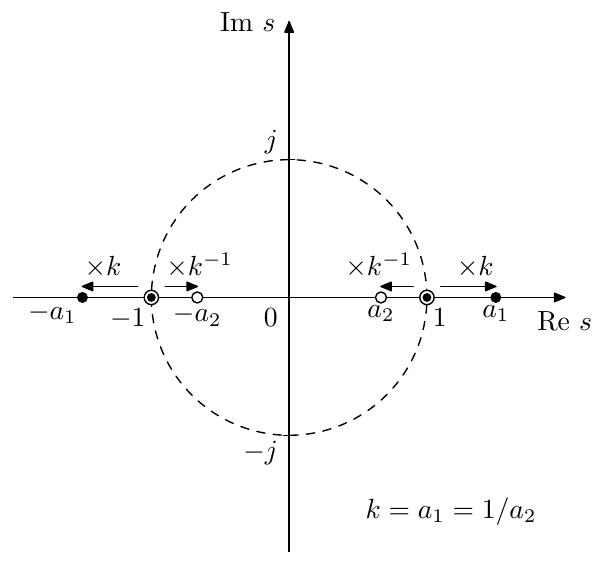
Figure 8.18: Roots of for (black dots are roots of , white dots are roots of ) and their positions at (indicated by circled dots, where each such dot denotes a root of coinciding with a root of ).
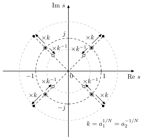
Figure 8.19: Roots of for (black dots are roots of , white dots are roots of ) and their positions at (indicated by circled dots, where each such dot denotes a root of coinciding with a root of ). Butterworth transformation order .
Writing out the “amplitude response” we have
Respectively, our goal is to have
So how do we find the roots of and ? If (, ) then, as we just discussed, simply generates a set of the Butterworth roots of the 1st kind on the unit circle. Now if we replace with (corresponding to replacing with ) this means a rotation of by the angle (Fig. 8.20). This rotates all roots of by (Fig. 8.21). At the same time will be rotated by and respectively all roots of by .
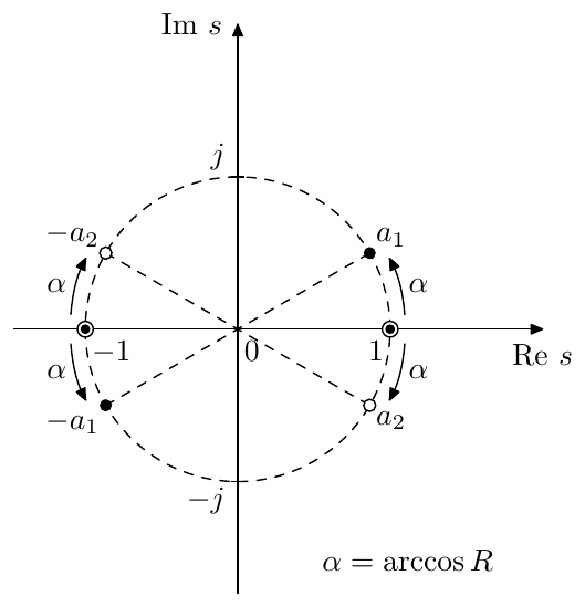
Figure 8.20: Roots of for (black dots are roots of , white dots are roots of ) and their positions at (indicated by circled dots, where each such dot denotes a root of coinciding with a root of ).
Even though generally for the set of roots of is not symmetric relatively to the imaginary axis and neither is the set of roots of , the combination of the two sets is symmetric (as one can observe from Fig. 8.21). Thus we can simply drop the roots in the right semiplane, the same way as we did for . Note that this also means that we do not need to rotate the full set of roots of and . Since at the end we are interested just in the left-semiplane roots, it suffices to rotate only the left-semiplane halves of the roots of and (that is, the roots of and ), as long as the roots do not cross the imaginary axis. It is not difficult to realize that the said crossing of the imaginary axis happens at corresponding to , where one of the roots on the imaginary axis will be from and the other from .
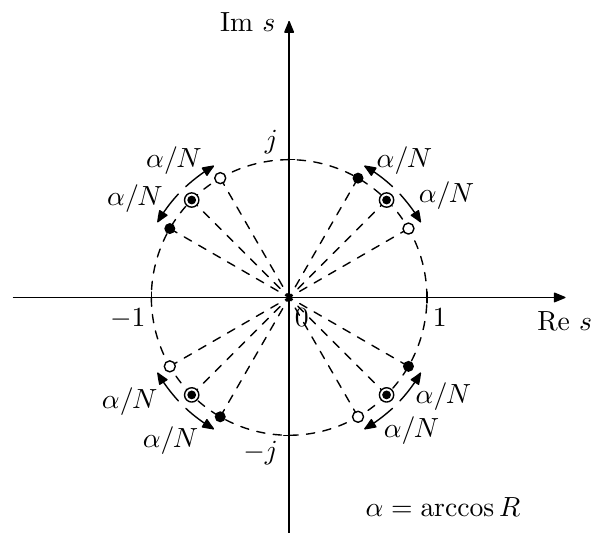
Figure 8.21: Roots of for (black dots are roots of , white dots are roots of ) and their positions at (indicated by circled dots, where each such dot denotes a root of coinciding with a root of ). Butterworth transformation order .
So, let’s reiterate. At () the roots of consist of two identical sets, each set being just the (left-semiplane) roots of a Butterworth transformation of a 1st-order polynomial , all roots in such set being located on the unit cicle. For we need to change the radii of both sets in a reciprocal manner:
(Fig. 8.19). For we need to rotate both sets by opposite angles
(Fig. 8.21).
We have mentioned that at () two of the rotated roots of reach the imaginary axis. Another special case occurs when the roots of are halfway from the “neutral position” () to selfoscillation (), that is when (). In this case the four roots of are equally spaced on the unit circle with the angular step . In the process of the Butterworth transformation we rotate the roots of and by , resulting in the set of roots of being equally spaced on the unit circle by the angular step . But this is the set of roots of the Butterworth transformation of the 1st kind of order (which produces the same polynomial order as the order Butterworth transformation of the 2nd kind). This result becomes obvious if we notice that at and the polynomial is the result of the Butterworth transformation of the 1st kind of order 2 of the polynomial . It is therefore no wonder that a Butterworth transformation of order 2 followed by a Butterworth transformation of order is equivalent to the Butterworth transformation of order (in other words, shrinking along the frequency axis by the factor is equivalent to shrinking first by the factor of 2 and then by the factor of ).
Seamless transition at
In the derivation of the Butterworth transformation of the 2nd kind we have been treating the cases and separately. In practice however we would like to be able to smoothly change from to and back in a seamless way (without clicks or other artifacts arising from an abrupt reconfiguration of a filter chain). This means that we need to find a way to distribute the roots of among 2nd-order factors in a continuous way, where there are no jumps in the values of the coefficients of these factors if is varied in a continuous way. Formally saying, the coefficients of the 2nd-order factors must be continuous functions of everywhere. The continuity for should occur for granted, thus we are specifically concerned about continuity at .
First, let’s assume the order of the transformation is even.
Let . There is an even count of the roots of and these roots come in complex-conjugate pairs (Fig. 8.19). Therefore each conjugate pair of roots of can be grouped into a single 2nd-order factor. The same can be done for and this half of our second-order factors corresponds to and the other half to .
At both sets of 2nd-order factors become identical, since becomes identical to .
At the roots of are rotated counterclockwise and the roots of are rotated clockwise (Fig. 8.21), therefore the roots of each of the polynomials won’t combine into conjugate pairs and thus the polynomials won’t be real anymore (Fig. 8.22).
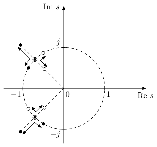
Figure 8.22: Movement of roots of (black dots) and (white dots) as smoothly varies around .
However, since we started the rotation from two identical sets of roots with conjugate pairwise symmetry within each set, for each root of there is now a conjugate root in and vice versa. We can therefore formally redistribute the roots between and in such a way, that the roots will be rotated by towards the negative real semiaxis (compared to ) and the roots will be rotated by away from the negative real semiaxis (Fig. 8.23).
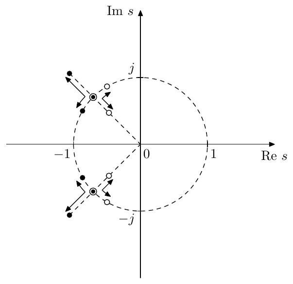
Figure 8.23: Movement of redistributed roots of (black dots) and (white dots) as smoothly varies around .
Thus, at we have two identical sets of roots. At the roots of move outwards from the unit circle, at the roots of move towards the negative real semiaxis. The roots of move inwards from the unit circle () and away from the negative real semiaxis (). This way we can keep the same assignment of the roots to the 2nd-order factors.15
If the order of the transformation is odd, then besides the conjugate pairs that we just discussed, we get two “special” roots, corresponding to the purely real root of the Butterworth transformation of the 1st kind of (Fig. 8.24). These two roots are real for and complex conjugate for , where at both roots are at . Thus, they can simply be assigned to one and the same 2nd-order factor of the form (which cannot be formally assigned to or , but can be thought of as being “shared” among and ), where depends on .
Arbitrary 2nd-order polynomials
The non-unit-cutoff polynomials can be simply treated using (8.12c).
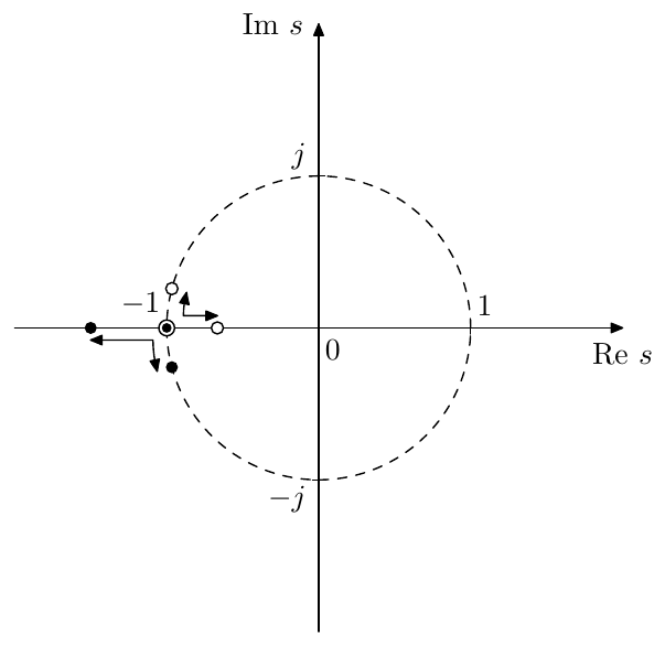
Figure 8.24: Movement of the “special” root of (black dot) and the “special” root of (white dot) as smoothly varies around .
The case can be taken in the limiting sense giving .
The case also can be taken in the limiting sense .
The case can be treated by noticing that the amplitude responses of and are identical. Thus, we can apply the Butterworth transformation to the positive-damping polynomial . Since the roots of in case of lie in the right complex semiplane, we might as well pick the right semiplane roots for . Particularly, if is the numerator of a maximum phase filter, the transformation result will retain the maximum phase property.
The polynomial of the most general form can be treated by rewriting it as where usually , . If then has two real roots of opposite sign and can be handled as a product of two 1st-order polynomials, to which we can apply Butterworth transformation of the 1st kind. If , we can treat this as a limiting case . Noticing that at the damping we rewrite as a product of real 1st-order terms:
and as vanishes we discard the infinitely large root of the polynomial (and the associated roots of ), formally replacing the polynomial with the constant factor .
Lowpass Butterworth filter of the 2nd kind
Given
and transforming its denominator according to the previous discussion of the Butterworth transformation of a 2nd order polynomial we obtain
Therefore can be implemented as a series of 2-pole lowpass filters.
Fig. 8.25 compares the amplitude response of a Butterworth lowpass filter of the 2nd kind () against the prototype resonating 2-pole lowpass filter. Note the increased steepness of the cutoff slope and the fact that the resonance peak height is preserved by the transformation.
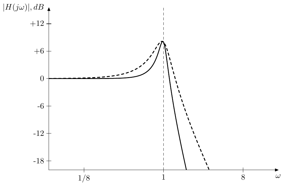
Figure 8.25: 4th order lowpass Butterworth filter of the 2nd kind vs. 2nd order lowpass filter (dashed line).
Fig. 8.26 compares the same Butterworth lowpass filter against cascading of identical 2nd order lowpasses, where the resonance has been adjusted to maintain the same resonance peak height. Note the much larger width of the resonance peak of the latter.
As mentioned before in the discussion of the Butterworth transformation of the 2nd kind, at we get the same set of poles as for order Butterworth transformation of the 1st kind. Thus, at this resonance setting our lowpass Butterworth filter of the 2nd kind (the filter order of which is ) is equal to the lowpass Butterworth filter of the 1st kind of the same filter order .
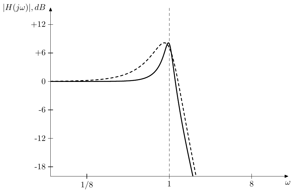
Figure 8.26: 4th order lowpass Butterworth filter of the 2nd kind vs. duplicated 2nd order lowpass filter of the same resonance peak height (dashed line).
Highpass Butterworth filter of the 2nd kind
The highpass Butterworth filter of the 2nd kind is obtained from
resulting in
Therefore can be implemented as a series of 2-pole highpass filters. Fig. 8.27 shows the respective amplitude response.
As with lowpass Butterworth filter of the 1st kind, the highpass Butterworth filter of the 2nd kind can be equvalently obtained by applying the LP to HP substitution to a lowpass Butterworth filter of the 2nd kind.
As with lowpass Butterworth filter of the 2nd kind, at we get a highpass Butterworth filter of the 1st kind.
Bandpass Butterworth filter of the 2nd kind
The bandpass Butterworth filter of the 2nd kind is obtained from
resulting in
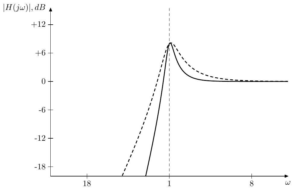
Figure 8.27: 4th order highpass Butterworth filter of the 2nd kind vs. 2nd order highpass filter (dashed line).
Therefore can be implemented as a series of 2-pole bandpass filters. Differently from the bandpass Butterworth filter of the 1st kind, this one allows to control the amount of resonance. Fig. 8.28 shows the respective amplitude response.
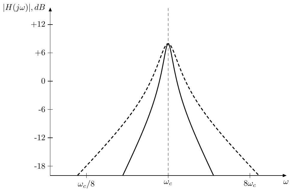
Figure 8.28: 4th order bandpass Butterworth filter of the 2nd kind vs. 2nd order bandpass filter (dashed line).
As with lowpass and highpass, at we get a bandpass Butterworth filter of the 1st kind. Since bandpass Butterworth filter of the 1st kind occurs only for an even transformation order , any bandpass Butterworth filter of the 1st kind is simply a bandpass Butterworth filter of the 2nd kind (of the same filter order ) at a particular resonance setting.
By replacing the underlying 2-pole bandpasses with their normalized versions one can obtain the normalized bandpass Butterworth filter of the 2nd kind:
One can of course also apply the LP to BP substitution to a Butterworth lowpass of the 2nd kind. Note, however, that if the lowpass has a resonance peak, then the resulting bandpass will have two of those, so this would be a rather special kind of a bandpass.
8.8 Generalized ladder filters
Now that we have learned to construct generic higher-order filters with resonance (by means of Butterworth transformation) we might consider going into the selfoscillation range by letting the 2nd kind Butterworth poles in Fig. 8.21 rotate past the imaginary axis (that is by letting ). Clearly we would need a nonlinear implementation structure then, to prevent the selfoscillating filter from explosion.
So far we have discussed 3 different implementations of generic high-order filters: generalized SVF and serial and parallel cascades. The SVF structure doesn’t accomodate nonlinearities easily, even though there can be ways. With serial and parallel cascades we of course could use various nonlinear 2-poles (and possibly nonlinear 1-poles) in the implementation, however this doesn’t feel very natural, compared to the nonlinearities appearing in the ladder filters. As we should remember, in ladder filters the resonance is created by the feedback, the more feedback, the more resonance, so that a saturator in the feedback loop was an efficient way to build a nonlinear ladder filter. In such filter the nonlinearity is a part of a feedback loop going through the entire filter, whereas in cascade implementations different nonlinearities would be independent. Of course, both approaches work in a way, but the approach where we have independent nonlinearities feels somewhat more artificial than the one with a “global” nonlinearity affecting the entire filter. For that reason we will make another attempt at generalizing the 4-pole ladder filter to abitrary pole counts.
We have seen that one can apply the general idea of a ladder filter to pole counts other than 4 by simply increasing the number of underlying 1-poles, but it hardly looks as a smooth generalization, as, except for bandpass16 ladders, the resonance behavior of the resulting filters is obtaining “special features”, like e.g. an offset of the resonant peak position for the 8-pole lowpass. We will start now with a different approach, namely with the generalized SVF (Fig. 8.1) where we replace all integrators with 1-pole lowpass filters (which, as it’s not diffiult to realize, corresponds to the substitution ). Fig. 8.29 illustrates (compare to Fig. 8.1).
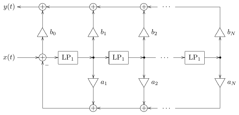
Figure 8.29: Generalized ladder (generalized TSK) filter.
Comparing to Fig. 5.9 we notice that the difference is that we are taking the feedback signal as a linear combination of all modal outputs, rather than simply from the last modal output. Comparing to Fig. 5.26 we notice that the latter essentially implements the same idea: taking a mixture of modal outputs as feedback signal, where both structures become equivalent at and . Thus, one could see Fig. 8.29 also as a generalization of the TSK filter.
The transfer function of Fig. 8.29 can be obtained from the transfer function of Fig. 8.1 by substitution:
Given a prescribed transfer function in the usual form
we could obtain the and coefficients from and by equating both transfer function forms
and then performing the (or equivalently ) subtitution on the entire equation:
Now we simply expand all in the right-hand side and equate the coefficients at the same powers of to obtain the expressions for and via and .
Nonlinearities
Letting all in Fig. 8.29 we obtain an -th order lowpass of the form . This consideration shows that the resonance in Fig. 8.29, if any, would be created through non-zero coefficients and one could prevent the filter from exploding selfoscillation by inserting a saturator into the feedback path, which would effectively reduce the values of , bringing them almost to zero at excessive signal levels. Fig. 8.30 illustrates.
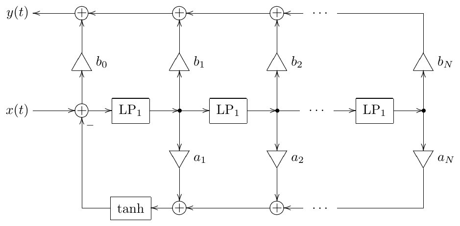
Figure 8.30: Nonlinear generalized ladder.
The feedback modal mixing coefficients serve the role of the feedback gain coefficient from Fig. 5.9. That is we don’t have anymore a single gain coefficient to control the feedback amount. Therefore we can’t place the saturator in Fig. 8.30 before the gains. If a reverse placement of the saturator relatively to the gains is desired, we can use the transposed version of Fig. 8.30.
In order to compare Fig. 8.31 to Fig. 5.9, or, even better, this time to Fig. 5.1 we should assume in Fig. 8.31 all except , which corresponds to modal gains for the pure -th order lowpass mode. Then we can see that Fig. 8.31 differs from Fig. 5.1 by the fact that the feedback is going not only to the input of the first lowpass stage, but to all lowpass stages. It is also instructive to compare Fig. 8.31 to Fig. 5.31, where we should be able to see that Fig. 8.31 is a generalized version of Fig. 5.31 with and .
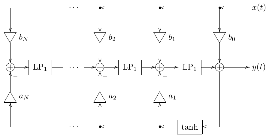
Figure 8.31: Transposed nonlinear generalized ladder.
Non-lowpass generalizations
In principle we could perform other substitutions in the generalized SVF structure. E.g. we could replace integrators with highpass filters, which corresponds to the substitution or, equivalently . This would correspond to generalized highpass ladder filters. More complicated substitutions could also be done, e.g. replacing some integrators with highpasses and some with lowpasses. One also doesn’t have to be limited by using 1-poles as substitutions. Having outlined the basic idea, we won’t go into further detail.
Summary
We have introduced four general topology classes: the generalized SVF, the serial cascade form, the parallel form and the generalized ladder filter. These topologies can be used to implement almost any transfer function (with the most prominent restriction being that the parallel form can’t deal with repeated poles).
We also introduced two essentially different ways to obtain a higher-order filter from a given filter of a lower order: identical filter cascading and Butterworth transformation. The former is stretching the amplitude and phase responses vertically (which may cause a number of unwanted effects), while the latter is shrinking the amplitude response horizontally.
-
Serial cascade implementation is especially popular in classical DSP, since direct forms commonly used there are reportedly starting to have more issues as the filter order grows, although the author didn’t verify that by his own experiments. ↩
-
Of course a multimode TSK, a multimode SKF, or any other 2nd-order filter with sufficient freedom in transfer function parameters would do instead of an SVF. ↩
-
Apparently can be implemented by 1-poles and SVFs if its factors can be implemented by 1-poles and SVFs. Those which can not, can be implemented by generalized SVFs. ↩
-
The idea to specifically address this is the book arose from a discussion with Andrew Simper. ↩
-
Denominators not achievable by classical SVFs can be achieved by using generalized 2nd- order SVFs. ↩
-
Of course, we could instead let and control the transfer function numerator by the input gains , or distribute the control between and . ↩
-
The dual approach would be to let the output mixing vector , in which case we control the transfer function’s numerator by the input gains. ↩
-
We can do this using formulas (4.7) and (4.8). ↩
-
The term Butterworth transformation has been coined by the author and is originating from the fact that this transformation, when applied to 1-pole filters, generates Butterworth filters. At the time of the writing the author is not aware of this concept being described elsewhere in the literature and would be thankful for any pointers to the commonly used terminology, if any exists. ↩
-
Of course, (8.11) doesn’t uniquely define . E.g. if satisfies (8.11), then so does . In that sense Butterworth transformation is not uniquely defined. However during the development of the Butterworth transformation we will suggest some default choices which will work most of the time. Assuming these default choices, the Butterworth transformation becomes uniquely defined. ↩
-
If is the numerator of a transfer function, then the roots all being in the left semiplane imply the minimum phase implementation. However in this case we could instead pick up the right semiplane roots as the roots of , thereby obtaining a maximum phase transfer function. Or one could take the minimum phase implementation and exchange one conjugate pair of roots of against the matching conjugate pair of roots of . Or one could exchange several of such pairs. Or one could exhange the real roots of and if the transformation order is odd. Still, the default choice will be to take the roots from the left semiplane. ↩
-
Obviously would also ensure . However, the default choice will be . ↩
-
Treating as a limiting case (here and later in the text) is important because it ensures the continuity of the result at the limiting point. ↩
-
With Butterworth transformation of the 2nd kind we won’t be making a distinction between even and odd roots. Instead we will be paying attention to which roots originate from and which from . ↩
-
Of course we could have done the opposite redistribution of roots among and , where the roots of move outwards from the unit circle and away from the negative real semiaxis, while the roots of move inwards from the unit circle and towards the negative real semiaxis. ↩
-
And allpass, as covered in Chapter 11. ↩