Chapter 7: State-space form
Starting with this chapter we begin the discussion of subjects of a more theoretical nature, not in the sense that they are not useful for practical purposes, but rather that one can already do a lot without the respective knowledge. Simultaneously the mathematical level of the presented text is generally higher than in the previous chapters. Readers who are not too interested in the respective subjects may consider skipping directly to Chapter 11, where the discussion returns to the previous “practical” level.
Transfer functions fully describe the behavior of linear time-invariant systems, but, as we already have seen, once the system parameters start to vary, we find out that some important information about the system topology is lacking. The state-space form provides a mathematical way to describe a system without losing the essential information about the system’s topology.1 Practically it’s not much different from block diagrams, just instead of a graphical representation of a system we represent it by mathematical equations. The state-space form can help to obtain new insights into the way how differential and difference systems work.
7.1 Differential state-space form
The term state-space form simply means that a differential system is written in the form of ordinary differential equations of the first order, where the differentiation is done with respect to time, and the equations have been algebraically resolved in respect to derivatives. E.g. suppose we are interested in a 2-pole allpass based on the state-variable filter (Fig. 4.1). In principle we already have the respective equations in (4.1) but for the sake of demonstration let’s reobtain them from the block diagram in Fig. 4.1.
Let denote the output of the first integrator and denote the output of the second integrator. The input of the first integrator is , thus
The output of the second integrator is simply :
According to (4.23), the allpass signal can be obtained as :
Writing all three equations together:
we have obtained the state-space form representation of Fig. 4.1, except that we are having integral rather than differential equations. From the mathematical point of view this is no more than a matter of notation and we can equivalently rewrite the same equations as
It is common to write the state-space equations in the matrix form:
or, by introducing
we rewrite the same in vector notation:
This is the general state-space form for a single-input single-output differential system. We can promote it further to multiple inputs and multiple outputs by promoting and to vectors and promoting , and to matrices:
E.g. for a single-input multiple-output LP/BP/HP SVF the equation (7.1b) turns into
The term state-space form originates from the fact that the vector of differential variables represents the states of the integrators, or simply the state of the system. Respectively the linear space of vectors is referred to as the state space of the system.
The state-space form encodes the essential information about the system’s topology, namely, which gains precede the integrators and which follow the integrators. Specifically, is the matrix of gains occuring on the paths from the inputs to the integrators, is the matrix of gains occurring on the paths from the integrators to the outputs, is the matrix of gains bypassing the integrators and is the matrix of gains on the feedback paths, thus they simultaneously precede and follow the integrators.
Integral form
Equations (7.2) can be rewritten in the integral form, which is merely a notational switch:
The integral form also allows to convert the state-space form back to the block diagram form. Each line of (7.3a) corresponds to an integrator, the respective right-hand side describing the integrator’s input signal.
Nonlinear state-space form
The right-hand sides of the equations (7.2) actually can be arbitary nonlinear vector functions of vector arguments, in which case we could write the equations as
The discussion of nonlinear systems has been done in Chapter 6. Most of the ideas discussed in Chapter 6 can be equally applied to the systems expressed as a state-space form, and we won’t discuss nonlinear state-space forms further.
7.2 Integratorless feedback
Before we can convert a block diagram (or an equation system, for that matter) into a state-space form we need to resolve integratorless feedback loops, if there are any. Integratorless feedback is a continuous-time version of zero-delay feedback. While zero-delay feedback loops in discrete time systems are the loops containing no unit delays, integratorless feedback loops in continuous time systems are the loops containing no integrators.
The resolution of integratorless feedback is therefore subject to the same considerations and procedures as the resolution of zero-delay feedback. We are going to demonstrate this using the TSK allpass from Fig. 5.35 as an example.
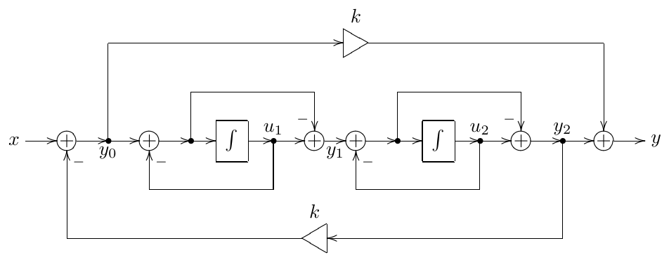
Figure 7.1: Allpass TSK filter from Fig. 5.35 with expanded 1-pole allpass structures.
Expanding the internal structures of the 1-pole allpasses in Fig. 5.35 we obtain the structure in Fig. 7.1. Denoting the 1-pole allpass states as and , their output signals as and and the input of the first 1-pole allpass as (as shown in Fig. 7.1) we obtain the following equations:
where this time we have assumed for simplicity.
Apparently Fig. 7.1 contains an integratorless feedback loop, starting at , going through the highpass path of the first allpass to , then through the highpass path of the second allpass to and returning via the global feedback path to . This loop contains three inverters and a gain of , thus the total gain of this integratorless feedback loop is and it is not instantaneously unstable provided . Under this assumption we can resolve it algebraically. Selecting just the equations for we have
We would like to solve for , therefore we first eliminate in the third equation:
and then in the just obtained equation:
and
Notice that the denominator corresponds to the instantaneously unstable case occuring for .
Now that we have resolved the integratorless feedback, we need to substitute the resolution result into the remaining equations of the original equation system:
Or, in the matrix form
7.3 Transfer matrix
If , all other signals in the system have the same exponential form and the system turns into
or
The first of the two equations is a linear equation system in a matrix form in respect to the unknown and the solution is found from
(where is a short notation for where is identify matrix), and
and thus
Introducing the matrix
we have
Thus is the transfer matrix of the system, its elements being the individual transfer functions corresponding to all possible input-output pairs of the system. In case of a single-input single-output system reduces to a matrix:
being simply the familiar transfer function.
From the formula (7.6) or (7.7) we can derive why the transfer functions of system built on integrators are nonstrictly proper rational functions. Indeed, the elements of are polynomials of of up to -th order (where is the dimension of the state space, that is simply the number of integrators). On the other hand, is a polynomial of of -th order. Therefore, the elements of are rational functions of sharing the same -th order denominator and having numerators of up to -th order. Thus, if , the elements of are strictly proper rational functions.
If , (7.6) turns into
and thus the numerators of the elements of become polynomials of order , if the respective element of matrix is nonzero. Thus, the transfer function becomes nonstrictly proper only if there is a direct (in the sense that it contains no integrators) path from the input to the output.
Note that, since the denominator of the transfer function(s) is , it follows that the roots of the polynomial are the system poles. At the same time the roots of are the eigenvalues of . Thus, eigenvalues of are the system poles.
7.4 Transposition
Computing the transfer matrix transpose we obtain from (7.6):
This looks like a transfer function of another system:
where
We will refer to this new system as transposed system. The transposition of the state-space form corresponds to the transposition of block diagrams described in Section 2.14. Particularly, we swap the input gains for the output gains and vice versa.
So, the transfer function of the transposed system is
where
or, in component form
while for the original system we have
But the input/output pair , , is the transposed system corresponds to the input/output pair , of the original system and the transfer function for each pair is . Thus, transposition preserves the transfer function relationships between the respective input/output pairs.
7.5 Basis changes
In the process of further analysis of state-space forms it will be highly useful to be able to change the basis of the state-space. Since a basis change is equivalent to a linear transformation of the linear space, let denote such transformation (where is some nonsingular matrix). Remember that what we are doing is changing the basis of the space, the transformation is just a way to notate the respective change of coordinates! Then and we can rewrite (7.2a) in terms of :
Respectively, (7.2b) in terms of turns into
Introducing
we obtain
which has exactly the same form as (7.2). That is we have obtained a new state-space representation of the system in the new basis. Note that thereby we didn’t change the basis of the spaces of the input signals or the output signals , but solely the basis of the state signals . Thus, the basis change is a purely internal operation and doesn’t affect the components of the vectors and . Respectively, the transfer matrix is not affected either, which can be explicitly shown by computing the transfer matrix in the new basis:
7.6 Matrix exponential
Another tool which we will need is the concept of the matrix exponential. We define the matrix exponential by writing the Taylor series for an ordinary exponential:
and replacing with a matrix:
The properties of the matrix exponential are similar to the ones of the ordinary exponential, except that typically the commutativity of the involved matrices is required. Particularly, the following properties are derived from (7.11) in a straightforward manner, under the assumption and :
The value of is particularly easy to compute if is diagonal:
In this case formula (7.11) turns into parallel Taylor series for and we simply have
If is not diagonal, but diagonalizable by a similarity transformation , the value can be computed by noticing that matrix exponential commutes with similarity trasformation:
which allows to express via . The formula (7.12) is obtainable from (7.11) in a straightforward manner as well, where we also notice that (7.12) holds for any and , they don’t have to commute.
If is not diagonalizable, then Jordan normal form can be used instead. We are going to address this case slightly later.
7.7 Transient response
The differential state-space equation (7.2a) can be solved in the same fashion as we solved the differential equations for the 1-pole in Section 2.15. Indeed, the difference between (7.2a) and the Jordan 1-pole (2.21) is that the former has matrix form. Also in (7.2a) the input signal is additionally multiplied by the matrix , but that doesn’t change the picture essentially.
Repeating the same steps as in in Section 2.15, we multiply both sides of (7.2a) by the matrix exponential :
or
Noticing that
we rewrite the state-space differential equation further as
Integrating with respect to time from 0 to :
The formula (7.13) is directly analogous to (2.22). Further, assuming complex exponential (note that all elements of share the same exponential , just with different amplitudes) we continue as:
Comparing to the transfer matrix for defined by (7.5) we introduce the steady-state response
and therefore
where is the transient response.
Note that we have just explicitly obtained the fact (previously shown only for the system orders ) that, given a complex exponential input , the elements of the steady-state response will be the same complex exponentials , just with different amplitudes. An immediately following conclusion is that the steady-state signals , being linear combinations of and , are also the same complex exponentials . In fact, any other steady-state signal in the system, being a linear combination of and , is the same complex exponential .
In a fully analogous to the 1-pole case way we can show that (7.14) also holds for
in which case
Substituting (7.14) into (7.2b) we obtain
where
and
The latter confirms the fact that is the steady-state response.
7.8 Diagonal form
We have seen that the transient response part of the signals in the system consists of linear combinations of elements of the matrix . The elements of can be easily found if is diagonalized by a similarity transformation. However, instead of diagonalizing the matrix taken in isolation, it will be more instructive to consider this as diagonalization of the state-space system itself.
According to (7.2a), the matrix is an operator converting vectors from the state space into vectors in the same space. This, diagonalization of can be achieved by a specific choice of the state space basis, where the basis vectors must be the eigenvectors of . After the change of basis we are having exactly the same system, just expressed in different coordinates. In these coordinates the matrix becomes diagonal and its diagonal elements are eigenvalues of (which are basis-independent). Now recall that eigenvalues of are the same as the system poles. Therefore, a sufficient condition for the state-space system to be diagonalizable is that all of its poles are distinct.2
Thus, in a diagonalizing basis the elements of are simply the system poles:
and the system falls apart into a set of parallel Jordan 1-poles:
where are the rows of matrix (respectively are the input signals of the Jordan 1-poles), and are the columns of matrix .
Stability
We already know that the transient response of a 1-pole is an exponent (where is the exponent’s amplitude). Respectively, the transient response part of in (7.16b) is a linear combination of transient responses of the Jordan 1-poles:
That is, the elements of are linear combinations of exponents .
Now recall that is independent on the choice of basis and so must be its separation into steady-state and transient response parts. Note that this is in agreement with the fact that according to (7.15) the steady-state response depends only on the transfer matrix and thus is independent of the basis changes. This means that the fact that the elements of are linear combinations of exponents is also independent of basis choice. Respectively if and only if . Thus we have obtained the explanation of the stability criterion for linear filters which we introduced in Section 2.9 and have partially shown for lower-order systems.3
Transfer matrix
Computing the transfer matrix for the diagonal form we notice that
that is we have transfer functions of the Jordan 1-poles on the main diagonal. Respectively the main term of the transfer matrix is just a linear combination of the Jordan 1-pole transfer functions. Apparently the common denominator of the terms of this linear combination is
which is simultaneously the common denominator of the transfer matrix elements.
It can be instructive to explicitly write out the elements of the transfer matrix in the diagonal case:
that is, we are having a partial fraction expansion of the rational function into fractions of 1st order. Thus, if a transfer matrix is given in advance, there is not much freedom in respect to the choice of the elements of and . The poles are prescribed by the common denominator of the transfer matrix and the values of the products and of are prescribed by the specific functions occurring in the respective elements of the transfer matrix.
In the single-input single-output case the transfer matrix has dimensions, while has and has dimensions respectively. Thus there is only one equation (7.18) and we have freedom degrees in respect to the choice of and giving the required values of the products . Each such degree can be associated with a variable , where we replace with and with . Apparently such replacement doesn’t affect the value of the product . One can also realize that simply scale the levels of the signals , which corresponds to different choices of the lengths of the basis vectors.
Now if we add one more output signal, thereby the dimensions of becoming , we can notice that we still have exactly the same degrees of freedom. If we attempt to change any of we need to compensate this in both of for the same by dividing these by , the latter being the ratio of the new and old values of . Respectively, if we change any of in one of the two rows of , this immediately requires the compensating change of , which in turn requires that the same change occurs not just in one but in both rows of . Adding more rows to and/or more columns to we see that the available freedom degrees are still the same and correspond to the freedom of choice of the basis vector lengths.
Thus, aside from the free choice of the basis vector lengths (and of their ordering) the transfer matrix uniquely defines the diagonal form of the state- space system. Respectively, for a non-diagonal form, if the matrix is given, then the transformation to the diagonal form is uniquely defined (up to the lengths and the ordering of the basis vectors), and, since the transfer function uniquely defines the matrices , and of the diagonal form, the matrices , and are also uniquely defined.
Steady-state response
Apparently, there is the usual freedom in regards to the choice of the steady-state response arising out of evaluating the inverse Laplace transform of to the left or to the right of the poles of . The change of the steady- state response (7.15) depending on the choice of the inverse Laplace transform’s integration path in (7.15) to the left or to the right (or in between) the poles of poses no fundamentally new questions compared to the previous discussion in the analysis of 1- and 2-pole transient responses and results simply in the changes of the amplitudes of transient response partials.
Diagonalization in case of coinciding poles
Even if two or more poles of the system coincide, it still might be diagonalizable, if the eigenvectors corresponding to these poles are distinct. It might seem that this is the most probable situation, after all, what are the changes of two vectors coinciding, or at least being collinear? Without trying to engage ourselves into an analysis of the respective probabilities, we are going to look at this fact from a different angle.
Namely, given a diagonal state space form with some of the eigenvalues coinciding, we are going to have identical entires in the matrix , as one can easily see from (7.17). This means that the order of the common denominator of the elements of will be less than and respectively the order of the denominator of the transfer matrix will also be less than . This means that the effective order of the system is less than and the system is degenerate.
Thus, a non-degenerate system with coinciding poles cannot be diagonalized. In such cases we will have to use the Jordan normal form, which we discuss a bit later.
7.9 Real diagonal form
Given a state-space system we could decide to implement it in a diagonal form by first performing a diagonalizing change of basis and then implementing the obtained diagonal state space form. However, if the system has complex poles, the underlying Jordan 1-poles of the system will become complex too, respec- tively generating complex signals . So, while the system has real input and real output, internally it would need to deal with complex signals. Of course, in a digital world using complex signals internally in a system shouldn’t be a big problem. But, for one, this is simply unusual and complicates the implementa- tion structure. More importantly, operations on complex numbers are at least twice as expensible as the same operations on real numbers. We therefore wish to convert a diagonal form containing complex poles to a purely real system, while retaining as much of the diagonalization as possible.
Since the system itself and the matrix in the original basis are real, the complex poles need to come in conjugate pairs. Without loss of generality we can order the poles in such a way that complex-conjugate pairs come first, followed by purely real poles: (where , , etc.) We will refer to the complex poles as the odd poles and to , as the even poles. When referring to odd/even poles we will mean only the essentially complex poles, the purely real poles being excluded. Since the poles are eigenvalues of , we will be referring to even/odd eigenvalues and respectively to even/odd eigenvectors.
Let be the eigenvector corresponding to , that is . Then, since has purely real coefficients, , (where denotes conjugation of vector’s components). Thus is the eigenvector corre- sponding to . Obviously, the same applies to any other even/odd eigenvector. Therefore we can choose a set of eigenvectors such that even eigenvectors are component conjugates of odd eigenvectors: .
If is the diagonalizing transformation of the system, the new basis must consist of eigenvectors of . Respectively, since , the columns of must consist of the new basis vectors, that is of the eigenvectors of (or, more precisely, consist of coordinates of these eigenvectors in the original basis). We will choose
This means that applying component conjugation to swaps the even and the odd columns of , which can be expressed as
where
is the “swapping matrix”. Note that elements of are purely real and that .
Since
component conjugation and matrix inversion commute:
Reciprocating the leftmost and the rightmost expressions we have
That is, component conjugation of swaps its even and odd rows. Or, put in a slightly different way, the even/odd rows of are component conjugates of each other, and so are the even/odd columns of .
Let’s now concentrate on the first conjugate pair of poles. Taking the diag- onalized form equations (7.16) we extract those specifically concerning the first two poles:
(where we need to employ the prime notation (7.10) for the diagonalized form, since we explicitly used the diagonalizing transformation , thus the non-primed state referring to the non-diagonalized form).
Using (7.9) and recalling that the first two rows of are component con- jugates of each other, we must conclude that so are the first two rows of , that is . Recalling that the first two colums of are component conjugates of each other, we conclude that . On the other hand, writing out the first two rows of (7.13) in the diagonal case we have
Except for the initial state term, the right-hand side of the second equation is a complex conjugate of the right-hand side of the first one. Regarding the initial state term, practically seen, we would have the following situations
- the initial state would be either zero, in which case ,
- or it would be a result of some previous signal processing by the system, where previously to that processing the initial state would be zero, in which case and respectively .
Therefore, we can simply require that , and thus the output signals and of the first two Jordan 1-poles are mutually conjugate. Respectively, the contribution of and into in (7.19c), being equal to , turns out to be a sum of two conjugate values and is therefore purely real. Obviously, the same applies to all other complex conjugate pole pairs.
Thus, even equations of (7.16a) do not contribute any new information about the system and we could drop them, simply computing even state signals as conjugates of odd state signals: , , etc. At the same time we could rewrite the odd equations of (7.16a) explicitly using real and imaginary parts of the signals :
Therefore we can introduce the new state variables, taking purely real values:
and
Then (7.20) turn into
and the respective terms in (7.19c) turn into
Thus we have obtained a purely real system
We will refer to (7.23) as the real diagonal form. It represents the system as a set of parallel 2-poles (7.22) (and optionally additional parallel 1-poles if some of the system poles are real).
Note that the substitutions (7.21) are expressible as another linear transfor- mation where
Therefore the real diagonal form of the system is related to the original form by a change of basis, where the respective transformation matrix is .
Jordan 2-poles
The 2-poles (7.22) in the real diagonal form are fully analogous to the 1-poles occuring in the diagonal form. They will also occur in the real Jordan normal form. For that reason we will refer to them as Jordan 2-poles. They are also sometimes (especially in their discrete-time counterpart form) referred to as coupled-form resonators.
The key feature of the Jordan 2-pole topology is that in the absence of the input signal, the system state is spiralling in a circle of an exponentially decaying (or growing) radius. Indeed, recalling that equations (7.22) are simply separate equations for the real and imaginary components of a complex signal , we can return to using the equation (7.19a), which by letting and turns into
where we also dropped the indices and the prime notation for simplicity. Re- spectively
On the other hand
therefore
Equating the right-hand sides of (7.24) and (7.25), we obtain
or
from where
or
Thus the complex value is rotating around the origin with the angular speed , it’s distance from the origin changing as , thereby moving in a decaying spiral if , an expanding spiral if , or a circle if . Recalling that the state components of (7.22) are simply the real and imaginary parts of in the above equations, we conclude that the state of (7.22) in the absence of the input signal is moving in the same spiral trajectory.
Notably, the separation of into real and imaginary parts works only if the pole is complex.4
Transfer matrix
In order to obtain the transfer matrix of the real diagonal form we could first obtain the transfer matrices of the individual 2-poles (7.22). Concentrating on a single 2-pole, we write (7.22) as
where we ignored the input mixing coefficients (in principle we can understand this form in the sense that the input signals are picked up past the mixing coefficients , or as a particular case of being identity matrix). We could explicitly compute the matrix for the above system, or we could derive it “manually”, which is what we’re going to do.
Given , we have
Respectively
Attempting to eliminate , we multiply each equation by a different factor:
and add both equations together:
Respectively attempting to eliminate , we multiply each equation by a different factor:
and subtract the second equation from the first one:
Thus
and, since for this system the matrix is identity matrix,
Note that the denominator is the standard 2-pole filter’s transfer function denominator, written in terms of the pole. Indeed, the complex conjugate poles and of two complex Jordan 1-poles were combined into a Jordan 2-pole by means of a linear combination. Respectively the Jordan 2-pole has exactly the same poles.
Generalizing the result obtained in (7.26) to systems of arbitrary order, containing multiple parallel 2-poles, we conclude that the main diagonal of contains the matrices of the form
similarly to how the transfer functions of the Jordan 1-poles are occurring on the main diagonal of in (7.17). Thus has the form
where have the form (7.27).
Similarly to what we did in the diagonal case, in the real diagonal case we also would like to explicitly write out the elements of the transfer matrix . For the sake of notation simplicity we will write them out for the case of a matrix . First, let’s notice that
where are the elements of and where denotes the outer product of the -th column of by the -th row of . Then, for a real diagonal system we obtain:
where and are obtained by summing the respective products of the elements of and . Respectively, for higher-order systems we have
Since real diagonal form is nothing more than a linear transformation of the diagonal form, there are the same freedom degrees in respect to the choice of the coefficients of and matrices, corresponding to choosing the basis vectors of different lengths.
7.10 Jordan normal form
We have shown that if a non-degenerate system has coinciding poles, it is not diagonalizable. The generalization of the diagonalization idea, which also works in this case, is Jordan normal form. The process of diagonalization implies that there is a similarity transformation of the matrix which brings the matrix into a diagonal form. Such transformation might not exist. However, there is always a similarity transformation bringing the matrix into the Jordan normal form.
The building element of a matrix in the Jordan normal form is a Jordan cell. A Jordan cell is a matrix having the form
That is it contains one and the same eigenvalue all over its main diagonal, and it contains 1’s on the subdiagonal right below its main diagonal, all other elements being equal to zero.5 Respectively, a matrix in the Jordan normal form consists of Jordan cells on its main diagonal:
(where is the number of different Jordan cells), all other entries in the matrix being equal to zero.
Apparently the sizes of all Jordan cells should sum up to the dimension of the matrix . The total number of times an eigenvalue appears on the main diagonal of is equal to the multiplicity of the eigenvalue. Typically there would be a single Jordan cell corresponding to a given eigenvalue. Thus, if an eigenvalue has a multiplicity of 5, typically there would be a single Jordan cell of size containing that eigenvalue. It is also possible that there are several Jordan cells corresponding to the same eigenvalue, e.g. given an eigenvalue of a multiplicity of 5, there could be a and a Jordan cell containing that eigenvalue. If there are several Jordan cells for a given eigenvalue, the respective state-space system is degenerate, fully similar to the case of repeated poles in the diagonalized case.
It is easy to notice that, compared to the diagonal form, Jordan cells appear on the main diagonal instead of eigenvalues. A Jordan cell may have a size, in which case it is identical to an eigenvalue appearing on the main diagonal. If all Jordan cells have size Jordan normal form turns into diagonal form.
Similarly to diagonal form being unique up to the order of eigenvalues, the Jordan normal form is unique up to the order of Jordan cells. That is, the number and the sizes of Jordan cells corresponding to a given pole is a property of the original matrix . The process of finding the similarity transformation converting a matrix into Jordan normal form is not much different from the diagonalization process: we need to find a basis in which the matrix takes Jordan normal form, which immediately implies a set of equations for such basis vectors. More details can be found outside of this book.
Jordan chains
It’s not difficult to realize that a Jordan cell corresponds to a series of Jordan 1-poles, which we introduced in Section 2.15 under the name of a Jordan chain. So, now we should be able to understand the reason for that name.
Indeed, suppose is in Jordnal normal form and suppose there is a Jordan cell of size located at the top of the main diagonal of . Then, writing out the first rows of (7.2) we have
Note that except for the first line, the input signal of the respective 1-pole contains the output of the previous 1-pole. In Fig. 2.24 we had a single-input single-output Jordan chain, now we are having a multi-input multi-output one (Fig. 7.2).
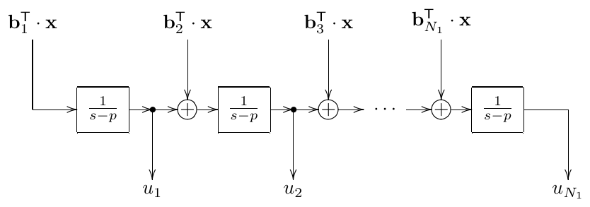
Figure 7.2: Multi-input multi-output Jordan chain
Transfer matrix
In the diagonal case the transfer matrix had a diagonal form (7.17) corresponding to the fact that the diagonal form is just a set of parallel Jordan 1-poles. Now we need to replace these 1-poles with Jordan chains. Thus, instead of single values on the main diagonal, the transfer matrix will have submatrices of the size of respective Jordan cells. From Fig. 7.2 it’s not difficult to realize that a transfer submatrix corresponding to a Jordan cell of the form (7.29) will have the form
Transient response
According to (7.13), the elements of the matrix are the exponent terms in which have the amplitudes . Apparently, being a part of the transient response, these terms do not explicitly depend on the system input signal and thus are the same in the single-input single-output and multiple-input multiple-output cases. Comparing to the explicit expression (2.25) for the output signal of a single-input single-output Jordan chain, we realize the following.
The elements of are . These elements are organized into submatrices of corresponding to Jordan cells of . Each such submatrix has the following form:6
This confirms that the stability criterion stays the same even if the system is not diagonalizable.
Real Jordan normal form
If the system has pairs of mutually conjugate poles, the Jordan cells for these poles will also come in conjugate pairs. Following the same steps as for diagonal form, we can introduce new state variables for the real and imaginary parts of complex state signals. Respectively, we each pair of conjugate Jordan cells will be converted to a purely real cell of double size. We will refer to such cells as real Jordan cells.
In order to understand how a real Jordan cell looks like, we can recall the interpretation of Jordan cells as Jordan chains (Fig. 7.2). Let’s imagine that the signals passing through this chain are complex. This can be equivalently represented as passing real and imaginary parts of these signals separately. Respectively, an element of a real Jordan chain must simply forward the real and imaginary parts of its output signal to the real and imaginary inputs of the next element. E.g. for a pair of conjugate 2nd-order Jordan cells
the corresponding real Jordan cell would be
7.11 Ill-conditioning of diagonal form
Suppose we are having a system where all poles are distinct, which is therefore diagonalizable. And suppose, as a matter of a thought experiment, we begin to modify the system parameters in a continuous way, simultaneously keeping track of the diagonal form of this system. We also keep track of the similarity transformation matrix defined by , where is the original state and is the “diagonalized” state. Note, that by this experiment we don’t mean that we are varying the system parameters in respect to time, rather we consider it as looking at different systems with different parameter values.
Suppose, we modify the system parameters in such a way, that some poles of the system get close to each other and finally coincide. Assuming the system order doesn’t degenerate, at this point we should switch from a diagonal matrix to a Jordan normal form matrix . The difference between these two matices is clearly non-zero, thus there is a sudden jump in the components of matrix at the moment of the switching. Respectively, there is a jump in the components of as well. We wish to analyse more closely, what’s happening in this case.
If two eigenvalues of a matrix become close then the respective eigenvectors might either also get close to each other or not. If they don’t, the eigenspace retains the full dimension as the poles coincide, respectively the system is diagonalizable and the system order degenerates. Thus, if the order of the system doesn’t degenerate, the eigenvectors corresponding to closely located eigenvalues must get close to each other too. Note that by saying that the eigenvectors are getting close to each other we mean that they are becoming almost collinear. Apparently, eigenvectors simply having different lengths but the same (or the opposite) directions don’t count as different eigenvectors.
Let’s pick a pair of such eigenvectors which are getting close to each other. Without loss of generality we may denote these two eigenvectors as and . In order to simplify the discussion, we will first assume that both eigenvectors are normalized: (where here and further the lengths will be defined in terms of the original basis, that is we are treating the original basis as an orthonormal one). Again, without loss of generality we may assume that and are pointing in (almost) the same direction.
Suppose we have a state vector lying fully in the two-dimensional subspace spanned by and . Therefore its coordinate expansion in the diagonalizing basis is a linear combination of and , the other coordinates being zeros:
We are going to show that and are not well defined.
Let’s introduce two other unit-length vectors into the same two-dimensional subspace:
Apparently, and are orthogonal to each other and we could expand in terms of and :
such expansion being well-defined, since the basis , is orthonormal.
Now we wish to express and via and :
from where
Since and are coordinates in an orthonormal basis, both and are taking values of comparable orders of magnitude, bounded by the length of the vector . On the other hand, since , the values of and will get extremely large, unless is very small.
Now consider a conversion from the basis , to a more “decent” basis, e.g. to , . Expressing , via , , we have
where and . Therefore
As we have noted, usually and are having very large magnitudes, while . This means that usually and are having opposite signs, in order to have , since . Respectively their difference is usually having a very large magnitude which is being compensated by the multiplication by .
Thus, the problematic equation is
where we add two very large numbers of opposite sign in order to obtain a value of of a reasonable magnitude. Such computations are associated with large numeric precision losses. Choosing different lengths for and will not change the picture, we still will need to obtain as the sum of the same opposite values of a much larger magnitude.
A conversion from the basis , to a “decent” basis other than , can be viewed as converting first to , and then to the desired basis. Apparently, converting from one “decent” basis to another “decent” one neither introduces new precision-related issues, nor removes the already existing ones.
Now realize, that essentially we have just been analysing the precision issues arising in the transformations from the original to the diagonalizing basis and back. It’s just that we have restricted the analysis to a particular subspace of the state space, but the transformation which we have been analysing was a diagonalizing transformation of the entire space. We have therefore determined that there are range and precision issues arising in the diagonalizing transformation when two eigenvectors become close to each other. We have also found out that this situation always occurs in non-degenerate cases of poles getting close to each other. Thus, diagonal form becomes ill-conditioned if the poles are located close to each other, the effects of ill-conditioning being huge precision losses and the values possibly going out of range. Jordan cells of size larger than 1 are nothing more than a limiting case of this ill-conditioned situation, where a different choice of basis avoids the precision issues.
The reader may also recall at this point the ill-conditioning in the analysis of the transient response of the 2-pole filters, which occurs at , when both poles of the system coincide on the real axis. That was exactly the same effect as the one which we analysed in this section.
7.12 Time-varying case
Until now we have been assuming that the system coefficients are not changing. If the system coefficients are varying with time, then quite a few of the previously derived statements do not hold anymore. This also causes problems with some of the techniques. The fact that the transfer function doesn’t apply in the time-varying case should be well-known by now, however the other issues arising out of parameter variation are not that obvious. Let’s look through them one by one.
Basis change
If the matrix is varying with time, we might need to vary with time as well, e.g. if is a matrix of the diagonalizing transformation. However, if is not constant anymore, the transformations of (7.8) get a more complicated form, since instead of
we are having
Thus (7.8) transforms as
respectively yielding
and
Thus the first of the equations (7.9) is changed into
The extra term in (7.30) is the main reason why different topologies have different time-varying behavior. If two systems are to share the same transfer function, they need to share the poles. In this case the matrices and have the same diagonal or Jordan normal form (unless the system order is degenerate) and are therefore related by a similarity transformation. Given that , and , are related via the same transformation matrix according to (7.9), the difference between the two systems will be purely the one of a different state-space basis, and we would expect a fully identical behavior of both. However, in order to have identical time-varying behavior, the matrices and would need to be related via (7.30) rather than via a similarity transformation. In fact (7.30) cannot hold, unless at least one of the matrices and depends not only on some externally controlled parameters (such as cutoff and resonance), but also on their derivatives, which is a highly untypical control scenario.
Transient response
In the derivation of the transient response in Section 7.7 we have been using the fact that
However if is not constant then the above needs to be written as
We might want to rewrite the derivative of as
but actually we cannot do that, since we don’t know whether the derivative of will commute with . Thus, our derivation of the transient response stops right there.7
Diagonal form
Given that we are using a diagonal form as a replacement for another non-diagonal system, we already know that such replacement changes the time-varying behavior of the system due to the extra term in (7.30).
A more serious problem occurs in this situation if we want to go through parameter ranges where the system poles get close or equal to each other. Such situation is unavoidable if we want a pair of mutually conjugate complex poles of a real system to smoothly change into real poles, since such poles would need to become equal on the real axis before they can go further apart. As we have found out, the diagonal form doesn’t support the case of coinciding poles in a continuous manner, since switching from poles to Jordan cells on the main diagonal is a non-continuous transformation of the state space.
Cutoff modulation
If all cutoff gains are identical and precede the integrators, it is convenient to factor them out of matrices and :
If the cutoff is varying with time, we could explicitly reflect this in the first equation, where we can also let (but not ) vary with time:
Introducing we have
or
where
Thus, as we have already shown in Section 2.16, cutoff modulation is expressible as a warping of the time axis, provided the cutoff is bounded to a finite positive range
where the time-warped system defined by (7.32) is time-invariant.
Note that cutoff modulation in (7.31) is a transformation of which changes its eigenvalues but not its eigenvectors. Thus, if we diagonalize the system by a basis change, the new basis can stay unchanged, and there will not be the extra term in (7.30). Respectively, the diagonalized system will stay fully equivalent to the original one, even though the cutoff is being modulated. Apparently the diagonalized system also can be written in the factored-out-cutoff form (7.31).
A somewhat more complicated reasoning can include the less restrictive case . Specifically, simply freezes the system state, while infinitely growing is not a problem as long as it doesn’t grow to infinity over a finite time range.
Equivalence of systems under cutoff modulation
It’s not difficult to realize that the equivalence under the condition of cutoff modulation in (7.31) holds not only between the original system and its diagonalized version, but between any two systems related by a basis change, since the cutoff modulation is not affecting the transformation between the two systems. Suppose we are having two systems sharing the same transfer function. In such case they have an equivalent behavior in the time-invariant case, but we wish to have it equivalent in the time-varying case too. More specifically, we would like to make the second system have the time-varying behavior of the first one.
Since the transfer function is the same, both systems share the same diagonal form up to the ordering and the lengths of the basis vectors. The transformations between both systems and the shared diagonal form are cutoff-independent and therefore the systems are equivalent.
Equivalence under other modulations
We have already shown that two systems sharing the same transfer function are equivalent under the cutoff modulation (7.31). We often would wish to also analyse for the equivalence under modulation of other parameters. Generally this will not be the case, but the state-space form techniques may allow us to find out more details about the specific differences between the systems. In order to demonstrate some of the analysis possibilities, we are going to analyse the TSK allpass (Fig. 7.1), which we have been converting to the state-space form in Section 7.2.
Taking (7.4) let’s replace the feedback amount with damping . From (5.17) we are having
and thus (7.4) turns into
Looking at the output mixing coefficients we notice a strong similarity to (4.23) where we subtract the bandpass signal (which, as we should remember, is obtained directly from one of the state variables of an SVF) from the input, the bandpass signal being multiplied by . On the other hand for the TSK allpass we have just obtained (7.33c):
This motivates to attempt an introduction of new state variables, where one of the variables will be a difference of and . We expect this variable to behave somewhat like an SVF bandpass signal.
Attempting to turn into exactly (which is what we would have had for an SVF) might be not the best idea, since the transformation would be dependent on , and it would be difficult to assess possible implications of such dependency. Instead we want something which is proportional to , but the transformation should be independent of . This is achieved by e.g.
which implies . Applying this transformation to (7.33) we have
from where
or
Now this looks very much like an SVF allpass, except that the input signal has been multiplied by and the bandpass signal is respectively multiplied by instead of multiplying by (Fig. 7.3). Note that the product of pre- and post-gains is still , exactly what we would normally use to build an SVF allpass. Thus, the only difference between the SVF allpass and the TSK allpass is the distribution of the pre- and post-bandpass gains.
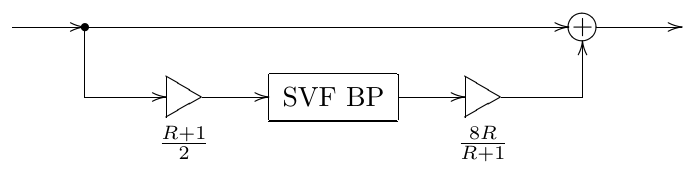
Figure 7.3: An equivalent representation of the allpass TSK filter from Fig. 5.35 using an SVF bandpass.
We could also cancel the denominator 2 of the pre-gain with the numerator of the post-gain (Fig. 7.4). Since 2 is a constant, “sliding” it through the SVF bandpass system effectively just rescales the internal state of the SVF by a factor of 2 (without introducing any new time-varying effects), but this rescaling is then compensated in the post-gain. Thus the system in Fig. 7.4 is fully equivalent to the one in Fig. 7.3.
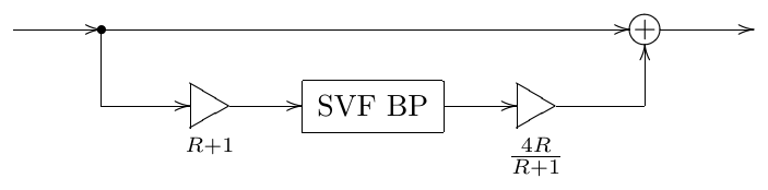
Figure 7.4: An equivalent modification of Fig. 7.3.
7.13 Discrete-time case
Discrete-time block diagrams can be converted to the discrete-time version of the state-space form, which is also referred to as the difference state-space form. The main principles are the same, except that instead of delivering the input signals of the integrators, it delivers the input signals of the unit delays. The same values will occur at the outputs of the unit delays one sample later, thus the first state-space equation takes the form
The second equation is the same as in the continuous-time case:
Writing both equations together we obtain the discrete-time state-space form:
Transfer matrix
Substituting the complex exponential signal into (7.34) we obtain
from where
From the first of the equations we have
Substituting this into the second equation we have
and thus
where
therefore the eigenvalues of are the system poles.
Transient response
Substituting the complex exponential input into (7.34a) we can rewrite (7.34a) as
or as
where
Recursively substituting (7.36) into itself at progressively decreasing values of we obtain
where
is the steady-state response (compare to the transfer matrix for in (7.35)), respectively
The generalization to arbirary signals is done in the same way as in the continuous-time case. The steady-state and transient responses for are trivially obtained from those for .
Stability
Considering the transient response in (7.37), we could diagonalize the system by a change of basis. If diagonalization is successful, then it’s obvious than decays to zero if and only if and grows to infinity if . Since neither the system poles nor the decaying of the transient response to zero depend on the basis choice, we have thereby established the criterion of stability of discrete time systems.
The non-diagonalizable case can be handled by using Jordan normal form, where the discrete-time Jordan 1-poles of the Jordan chains will be stable if and only if .
7.14 Trapezoidal integration
Writing (7.31) in an integral form we have
On the other hand, expressing direct form I trapezoidal integration Fig. 3.8 in equation form we have
Applying (7.39) to the integral in (7.38a) we obtain
from where
and
Equation (7.40) is the resolved zero-delay feedback equation for the state-space form (7.31) (or, equivalently (7.38)). Since we have used direct form I intergators, it needs additional state variables for the storage of the previous input values, which we could have spared if direct form II or transposed direct form II integration was used.
Let’s apply trasposed direct form II integration (3.3) to the integral in (7.38a). Apparently, we have a notation clash, since in (3.3) the variable is an internal variable of the integrator. Notating this internal variable as and notating the input signals of the integrators as , and also not forgetting to introduce a non-unit sampling period , we obtain from (3.3) a set of equations:
Solving for we have
where are the previous states of the integrators, and respectively
and
Equation (7.41) is another variant of the resolved zero-delay feedback equation (7.40), this time written for transposed direct form II form. The benefit, compared to (7.40), is that we only need to store the previous states of the integrators .
Since , the denominator of both equations (7.40) and (7.41) is . Since is the eigenvalue equation, the denominator turns to zero when 1 becomes an eigenvalue of , or respectively when becomes an eigenvalue of . Thus, we have a limitation
under which the system doesn’t get instantaneously unstable. Apparently are simply the poles of the system, thus (7.42) simply states that the real poles of the system must be located to the left of .8
Summary
The state-space form essentially means writing the system as a differential (or difference, in the discrete-time case) equation system in a matrix form. Thereby we have a compact abstract representation of the system, which, differently from to the transfer function, doesn’t lose essential information about the time-varying behavior. A particularly useful way to approach the state-space form analysis is by diagonalizing the matrix, which essentially separates the effects of different poles of the system from each other.
-
Except in cases where continuous-time block diagrams contain instantaneously unstable integratorless feedback loops. ↩
-
A little bit later we will establish the fact that a system where some poles coincide is most likely not diagonalizable. ↩
-
Of course, exactly the same results would have been obtained if we simply computed the explicit form of the matrix exponential for the diagonal matrix . However then we would have missed the interpretation of the diagonalizing basis as the basis in which the system can be seen simply as a set of parallel 1-poles. ↩
-
This is strongly related to the appearance of Jordan normal form at the moment when two complex conjugate poles coincide on the real axis. ↩
-
Some texts place 1’s above the main diagonal. This is simply a matter of convention. One can convert from one version to the other by simply reindexing the basis vectors. ↩
-
The explicit form of an exponent of a Jordan normal form matrix can also be obtained directly from (7.11), but that approach is more involved and we won’t do it here. ↩
-
Notably, the same was the case for our transient response derivations for 1- and 2-pole cases, where we were assuming the fixed values of system parameters. Except for the 1-pole case, where the only available freedom degree in the matrix could be represented as the cutoff, leading to an equivalent representation of the modulation via time-warping. ↩
-
Of course if there are complex poles sufficiently close to the real semiaxis , the performance of trapezoidal integration is also questionable. ↩