Chapter 6: Nonlinearities
The filters which we were discussing until now were all linear. Formally this means that if we consider a filter as an operator, this operator is a linear one. Practically this meant that the structures of our filters were consisting of gains, summators and integrators. However, filters used in synthesizers often show noticeably nonlinear behavior. In terms of block diagrams, introducing nonlinear behavior means that we should add nonlinear elements to the set of our block diagram primitives.
Nonlinear filters have more complicated behavior and are capable of producing richer sound than the linear ones. Usually they exhibit complex overdriving effects, when driven with an input signal of a sufficiently high level. Another special feature of many nonlinear filters is their ability to increase the resonance beyond a formally infinite amount, entering the so-called self-oscillation.
6.1 Waveshaping
We just mentioned that in order to build non-linear filters we need to introduce nonlinear elements into the set of our block diagram primitives. In fact we are going to introduce just one new type of element, the waveshaper:
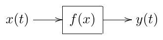
A waveshaper is simply applying a given function to its input signal, and sends the respective function value as its output signal:
The function can be any “reasonable” function, e.g. or etc.
Usually the function cannot vary with time, that is, the function’s parameters, if it has any, are fixed. E.g. if , then is usually fixed to some particular value, e.g. , which doesn’t vary. Often, this is just a matter of convention. e.g. the waveshaper can be represented as a serial connection of a gain element and the waveshaper itself:
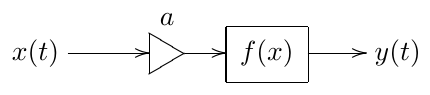
in which case the waveshaper itself is time-invariant.
Still, if necessary, it’s no problem for the waveshaper to contain time-varying parameters, as long as the time-varying parameters are “externally controlled” (in the same way how e.g. filter cutoff is controlled). That is, the waveshaper’s parameters cannot depend on the values of the signals within the block diagram. If one needs the parameter dependency on the signals of the block diagram, then one should consider such dependencies as additional inputs of the nonlinear element and we end up with a multi-input element of the block diagram. It is no problem to use such elements, but normally we should not refer to them as waveshapers, since commonly, waveshapers have one input and one output.
In order to be representable as a function of the input signal, a waveshaper clearly shouldn’t have any dependency on its own past. That is waveshaper is a memoryless element.
6.2 Saturators
The probably most commonly used category of waveshapers is saturators. There is no precise definition of what kind of waveshaper is referred to as saturator, it’s easier to give an idea of what a saturator is by means of example.
Bounded saturators
One of the most classical saturators is the hyperbolic tangent function:
(Fig. 6.1). Even if the input signal of this saturator is very large, the output never exceeds . Thus, this element saturates the signal, which is the origin of the term saturator.
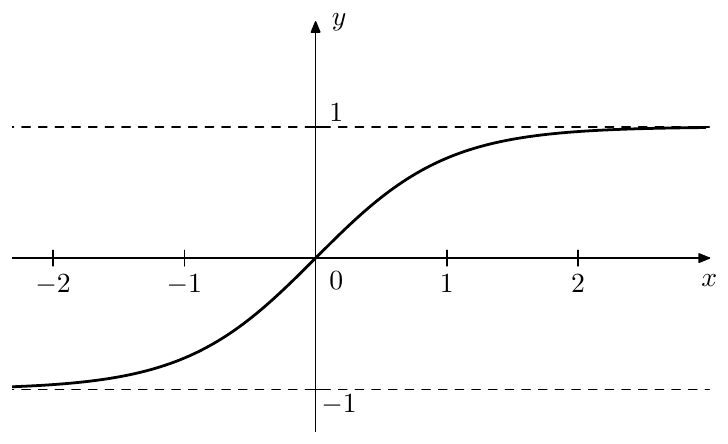
Figure 6.1: Hyperbolic tangent .
Other saturators with shapes similar to the hyperbolic tangent include:
(this list is by no means exhaustive). Is is not difficult to see that the values of the hyperbolic tangent (6.1) and the saturators (6.2) do not exceed 1 in absolute magnitude. That is, their ranges are bounded. We are going to refer to such saturators as bounded-range saturators or simply bounded saturators.
From the four introduced saturation functions the parabolic saturator (6.2b) stands out in that the full saturation is achieved at , whereas for other shapes it’s not achieved at finite input signal levels. Thus, the range of (6.2b) is , therefore being compact. We will refer to such saturators as compact-range monotonic saturators.
Another important distinction of the parabolic saturator is that it has three discontinuities of the second derivative (at and ) and the hyperbolic saturator has one discontinuity of the second derivative (at ). Even though such discontinuities are not easily visible on the graph, they affect the character of the saturator’s output signal. Usually such discontinuities are rather undesired, as they represent abrupt irregularities in the saturator’s shape, so it’s generally better to avoid those.1 A common reason to tolerate derivative discontinuities in a saturator, though, is performance optimization.
Transparency at low signal levels
A property commonly found with saturators is that at low levels of input signals the saturator is transparent: for . Equivalently this condition can be written as
Visually it manifests itself as the function’s graph going at through the origin. Clearly, all the previously introduced saturators have this property.
The property (6.3) is not really a must, but it’s quite convenient if the saturators have it, particularly for the analysis of system behavior at low signal levels. For that reason it’s common to represent a non-unit derivative at the origin via a separate gain. Given a saturation function such that but we introduce a different saturation function such that and . E.g. we can take
so that
The coefficient is then represented as a separate gain element.
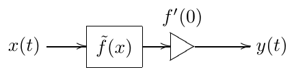
Apparently this representation is not available if , however in such cases the saturator effectively breaks the connection at low signal levels, working as a zero gain.
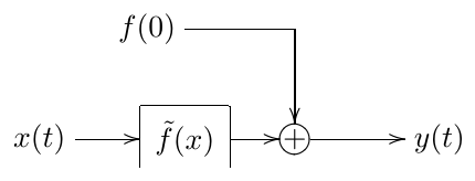
Saturators with can be represented by separation of the value into a DC offset signal:
which is treated as another input signal with a fixed value :
Unbounded saturators
Sometimes we want saturation behavior, but do not want a hard bound on the output signal’s level. One function with this property is inverse hyperbolic sine:
(Fig. 6.2) While having the usual transparency property (6.3), it is not bounded. The asymptotic behavior of the hyperbolic sine is similar to the one of the logarithm function:
Another saturator with a similar behavior can be obtained as an inverse of , which is
behaving as at .
Such kind of waveshapers are also referred to saturators, even though the saturation doesn’t have a bound. We will refer to them as unbounded-range or unbounded saturators.
Apparently, unbounded saturators represent a weaker kind of saturation than bounded ones. The weakest possible kind of saturation is achieved if grows as a linear function of at . Such saturators can be built by introducing a linear term into the saturator’s function. Given a saturator where can be any of the previously discussed saturators, we build a new saturator by taking a mixture of and :
where we needed to multiply by to keep the transparency property (6.3) (provided it was holding for ). Apparently for . We can refer to such saturators as asymptotically linear saturators. The previously discussed saturators such that for can be respectively referred to as slower-than-linear saturators.
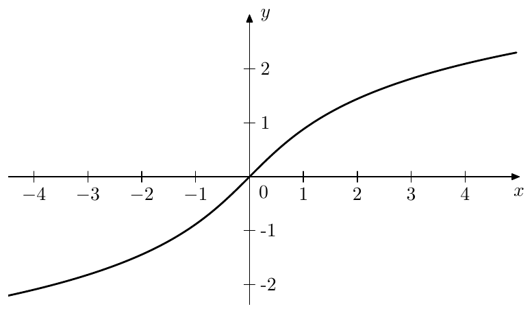
Figure 6.2: Inverse hyperbolic sine .
Soft- and hard-clippers
One special but important example of a saturator is the hard clipper, shown in Fig. 6.3.2 In contrast, we will be referring to all previously discussed saturators as soft clippers.3
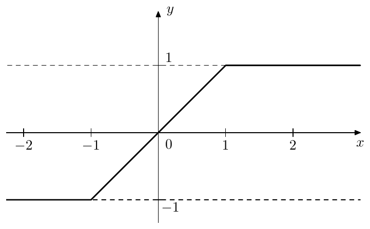
Figure 6.3: Hard clipper.
Saturation level
The previously introduced bounded saturators (6.1) and (6.2) were all saturating at . But that is not always desirable. Given a bounded saturator with the saturation level we can change the saturation level to by simultaneouly scaling the and coordinates:
(Fig. 6.4). The simultaneous scaling of and preserves the transparency property (6.3).
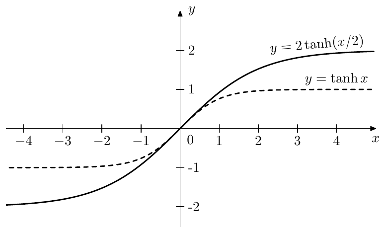
Figure 6.4: Changing the saturation level.
Saturator as variable gain
Sometimes it is useful to look at saturators as at variable gain elements. E.g. we can rewrite as
The graph of the function is shown Fig. 6.5. Thus
That is at low signal levels the saturator is transparent, at high signal levels is reduces the input signal’s amplitude by a factor of approximately . Apparently, this kind of behavior is shown by all bounded saturators. Unbounded saturators give a similar picture, as long as they are slower than linear. For asymptotically linear saturators, such as (6.6), we have instead.
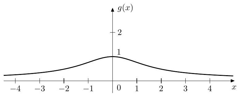
Figure 6.5: .
6.3 Feedback loop saturation
In the ladder filter and its variations, such as 4-pole and 8-pole ladders and SKF/TSK filters, the resonance is implemented by means of a feedback loop. By this we mean that when the feedback loop is disabled (by setting the feedback gain to zero), there is no resonance, and the resonance amount is increased by increasing the amount of the feedback (thus e.g. the SVF filter doesn’t fall into this category). With such filter structures, when the feedback amount goes above a certain threshold (e.g. for the 4-pole lowpass ladder or for the SKF) the filter becomes unstable and “explodes” (the filter’s state and the output signal indefinitely grow). By putting a saturator anywhere within such feedback loop we can prevent the signals in the feedback loop from the infinite growth, making the filter stable again.
Feedforward path saturation
One of the common positions for the feedback loop saturator is in the feedforward path right after the feedback merge point (Fig. 6.6). Given that the saturator is a bounded one (such as ), the output signal of such saturator is guaranteed to be bounded. Since the rest of the feedforward path in Fig. 6.6 is known to be BIBO-stable (independently of the feedback setting), the output of the filter is bounded too and thus the entire filter is BIBO-stable.
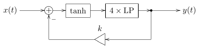
Figure 6.6: Ladder filter with a saturator in the feedforward path.
We could also view the saturator in Fig. 6.6 as a variable gain (6.8). Apparently, as the amplitude of the signal grows, the average value of is decreasing to zero. In those terms, the saturator is effectively reducing the feedback gain from to (where is the average value of ). Since at large signal amplitudes can get arbitrarily close to zero, the value of goes below 4, which, intuitively, prevents the filter from exploding. Unbounded saturators are therefore having the same effect, as long as they are slower than linear.
With asymptotically linear saturators the filter will still explode at some point. Assuming the saturator has the form (6.6) we have and thus and . Thus, we could expect that for something like the filter should not explode.
Effects of transient response
As we should remember, one possible way to look at a filter getting unstable is that its transient response grows instead of decaying with time. Each pair of conjugate poles and of the filter contributes a transient component of the form
Thus at we have a sinusoid of frequency . At we have the same sinusoid of an exponentially growing amplitude. This sinusoid will be present in the filter’s output even in the absence of the input signal.4 Since at this sinusoid is self-sustaining, the filter is said to self-oscillate. The saturator in the feedback loop prevents the self-oscillation from infinite growth.5
Suppose the system in Fig. 6.6 is at , that is it is selfoscillating or at least strongly resonating. Let
denote the input signal of the saturator and recall the representation of a saturator as a variable gain element (6.8). Then the output signal of the saturator is
where . Comparing (6.10) to the last expression in (6.11) we see that the effect of the saturator can be seen as the “replacing” with and with . Thus, is the new “effective feedback amount”. Now, by increasing the amplitude of the input signal we increase the amplitude of and thus reduce the magnitude of and thereby reduce the effective feedback amount , which in turn shows up as reduction of resonance. That is, at high amplitudes of the input signal the resonance oscillations kind of disappear.
One intuitive way to look at this is to say that the input signal and the resonance are “fighting” for the saturator’s headroom, and if the input signal has a very high level, it “pushes” the resonating component of the signal out. On the other hand, if the input signal level is low, then the entire headroom is taken by the resonating component which will be therefore much louder than the input signal. There is usually some “sweet spot” in the input signal’s level, where the fighting doesn’t kill the resonance, but results in a nice interaction between the input signal and the resonance.
Feedback path saturation
The amount of fighting (at the same input signal level) can be decreased by putting the saturator into the feedback path, either prior to the feedback gain (Fig. 6.7) or past the feedback gain (Fig. 6.8).6 In this case the input signal doesn’t directly enter the saturator but first goes through the four 1-pole lowpass filters, which somewhat reduces its amplitude (depending on the signal and on the filter’s cutoff). The difference between Figs. 6.7 and Fig. 6.8 is obviously that in one case the effective saturation function is whereas in the other one it’s . This means that in the first case the saturation level is whereas in the second one it’s fixed to (Fig. 6.9).
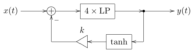
Figure 6.7: Ladder filter with a saturator in the feedback path (pre-gain).
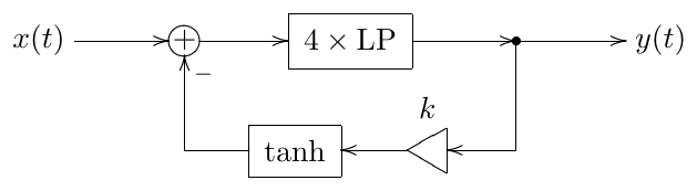
Figure 6.8: Ladder filter with a saturator in the feedback path (post-gain).
The amount of fighting will also be decreased by using a weaker saturation curve. E.g. using an unbounded saturator instead of a bounded one, in the most extreme case having an asymptotically linear saturator. A classical example of this approach is ecountered in the nonlinear Sallen-Key filter (Fig. 6.10). It is an interesting observation that the sound of nonlinear Sallen-Key filter significantly differs from the sound of nonlinear transposed Sallen-Key filter (Fig. 6.11) since in one case the saturator’s output goes through a highpass and a lowpass, while in the other case it goes through two lowpasses before reaching the filter’s output.7
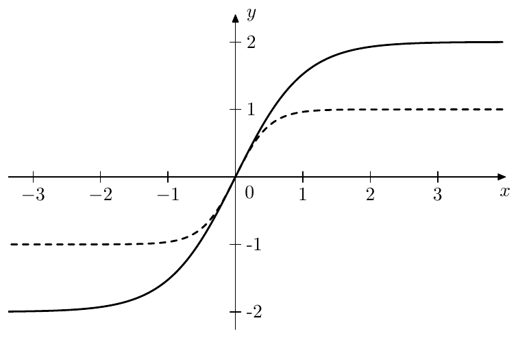
Figure 6.9: Pre-gain (, solid) vs. post-gain saturation (, dashed).
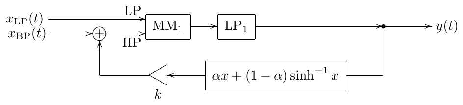
Figure 6.10: Sallen-Key filter with an asymptotically linear saturator.
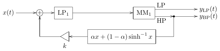
Figure 6.11: Transposed Sallen-Key filter with an asymptotically linear saturator.
Transfer function
For systems containing nonlinear elements the complex exponentials are no longer system eigensignals. That is, given an input signal of the form the output will not have a similar form. Therefore the idea of the transfer function as well as amplitude and phase responses doen’t work anymore.
Still, given that the nonlinear elements satisfy the transparency condition (6.3), at low signal levels the nonlinearities have almost no effect and the system is approximately linear. In that sense the transfer function stays applicable to a certain degree and still can be used to analyse the filter’s behavior, although the error is growing stronger at higher signal levels. Nevertheless, as a rule, qualitatively the filters retain their main properties also in the presence of saturators. The lowpass filters stay lowpass, bandpass filters stay bandpass etc.
6.4 Nonlinear zero-delay feedback equation
The introduction of the nonlinearity in the feedback path poses no problems for a naive digital model. In the TPT case however this complicates the things quite a bit. Consider Fig. 5.5 redrawn to contain the feedback nonlinearity (Fig. 6.12).
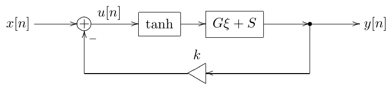
Figure 6.12: Nonlinear TPT ladder filter in the instantaneous response form.
Writing the zero-delay feedback equation we obtain
Apparently, the equation (6.12) is a transcendental one. It can be solved only using numerical methods. Also, the linear zero-delay feedback equation had only one solution, but how many solutions does (6.12) have? In order to answer the latter question, let’s rewrite (6.12) as
If then is a nonstrictly increasing function of ,8 while is a strictly decreasing function of . Thus, (6.13) (and respectively (6.12)) has a single solution (Fig. 6.13). At we also typically have one solution (Fig. 6.14) unless , in which case (6.13) has three solutions Fig. 6.15. Fortunately, corresponds to instantaneously unstable feedback, and thus normally we are not so much interested in this case anyway. However, if needed, one could use the concept of the instantenous smoothing to find out the applicable solution among the three formal ones.
Having found the zero-delay equation solution , we proceed in the usual way, first letting through the tanh waveshaper and then letting it through the 1-pole lowpasses (denoted as in Fig. 6.12), updating the 1-pole states along the way and ultimately obtaining the value of .
Now we are going to discuss some possible approaches for finding . This discussion is by no means exhaustive and the reader is advised to consult the literature on numerical methods for further information.
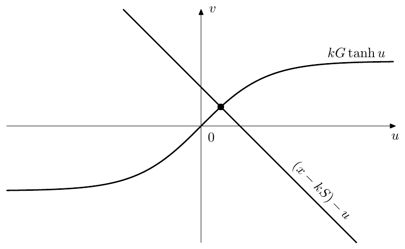
Figure 6.13: The solution of (6.13) for k > 0.
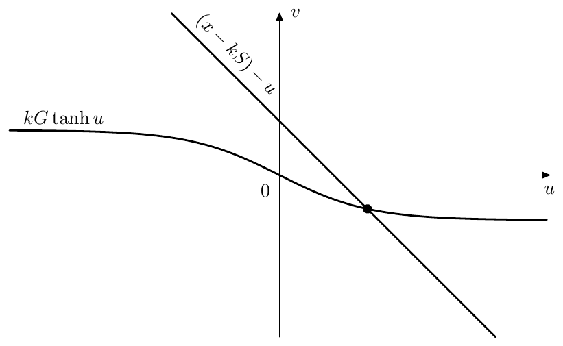
Figure 6.14: The solution of (6.13) for -1 < kG < 0.
6.5 Iterative methods
Fixed-point iteration
Starting with some initial value we compute iteratively the left-hand side of (6.12) from the right-hand side:
and hope that this sequence converges quickly enough.9 Intuitively, the convergence gets worse at larger absolute magnitudes of , that is at high cutoffs (large ) and/or high resonance values (large ). Conversely, it gets better as the sampling rate increases (since becomes smaller in this case). Generally, the convergence fails for .
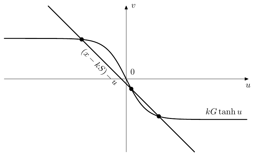
Figure 6.15: Solutions of (6.13) for kG < -1.
The process defined by (6.14) has a strong similarity to the naive approach to time discretization. Indeed, for the frozen values of and one can treat Fig. 6.12 as stateless zero-delay feedback system (Fig. 6.16). And then we simply implement this system in the naive way by introducing a unit delay at the point of the signal (Fig. 6.17) and letting this system run for some number of discrete-time ticks. This is a bit like oversampling of the instantaneous feedback loop part of the system.10
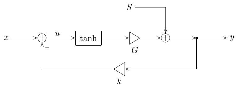
Figure 6.16: Zero-delay feedback equation (6.12) as a stateless zero-delay feedback system.
So, it is as if we introduce a “nested” discrete time into a single tick of the “main” discrete time. This suggests a natural choice of the initial value of for (6.14), namely, taking the previous value of (that is the value from the previous sample of the “main” discrete time) as the iteration’s initial value .
Under the consideration of the concept of the instantaneous smoothing (introduced in Section 3.13), the interpretation in Fig. 6.17 also suggests a way to improve the convergence of the method by introducing a smoother into the feedback loop of Fig. 6.17. In a practical implementation such smoother can be a naive 1-pole lowpass, like in Fig. 6.18, which effectively lowers the total feedback gain from to a smaller value.11 However, even though such smoother may improve the convergence at high , obviously it can deteriorate the convergence in good situations. Particularly at the iteration process is supposed to immediately converge, however in the presence of the lowpass smoother it will converge exponentially instead.
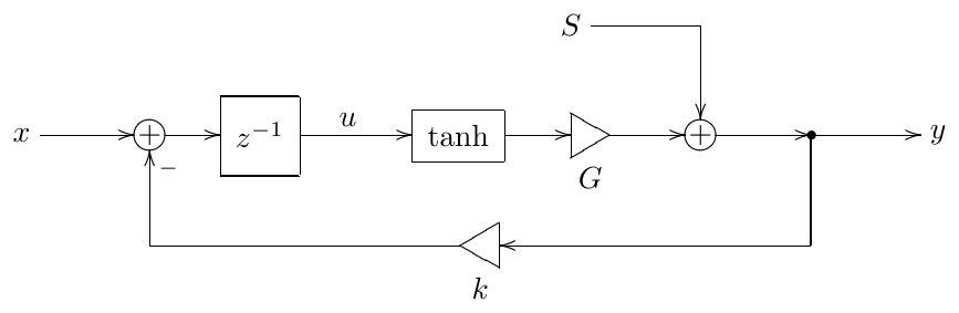
Figure 6.17: Interpretation of the equation (6.14) as an “oversampled” naive discrete-time model of the stateless feedback loop in Fig 6.16.
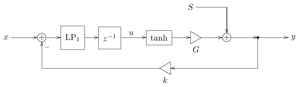
Figure 6.18: Using a 1-pole lowpass smoother to improve convergence of signals in Fig. 6.17.
Newton-Raphson iteration
A very popular approach in practical DSP is Newton-Raphson method, which is based on the idea of linearization of the function around the current point by the tangent line. Instead of solving (6.13) we solve
for to obtain the next guess and repeat the iteration (6.15) until it converges. Fig. 6.19 illustrates the idea.
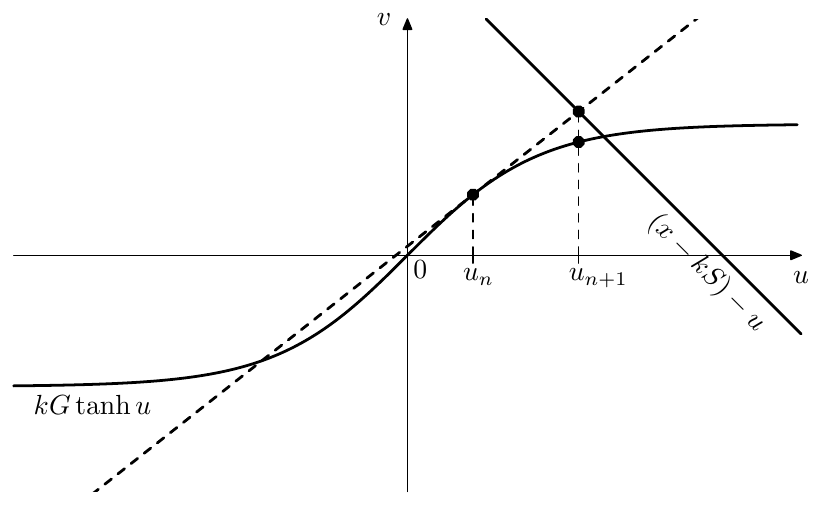
Figure 6.19: Newton-Raphson method: linearization by the tangent line.
The textbook version of Newton-Raphson method is formulated in terms of searching for a zero-crossing of a function (Fig. 6.20). By subtracting the left-hand side of (6.13) from the right-hand side we obtain the equation
Respectively, the iterations are generated by solving
Apparently (6.15) and (6.17) (and respectively Figs. 6.19 and 6.20) are equivalent, both giving
Newton-Raphson method converges very nicely in almost linear areas of , the convergence getting worse as becomes more nonlinear. As with fixed-point iteration, the convergence deteriorates at large , as the prediction error of increases.12
As in the fixed-point iteration method, the value of from the previous sample tick is a natural choice for the iteration’s initial value as well. This choice usually leads to fast convergence if the new solution lies close to the value of on the previous sample. However in excessive situations (such as high cutoff and/or high input signal frequency) the old solution could lie within the right-hand side saturation range of (that is ) and the new solution could lie within the left-hand side saturation range of (that is ).
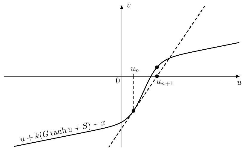
Figure 6.20: Texbook version of Newton-Raphson method (note that the aspect ratio of the graph is not 1:1)
The solution search by Newton-Raphson iterations will need to traverse both “knees” (areas of higher curvature) of tanh along the way, which usually has a negative impact on the convergence. The neutral choice of as initial value might somewhat improve this worst-case scenario, while simultaneously deteriorating the convergence in “nice” situation.
Other, more advanced approached to the choice of the initial point may be used. Often one uses Newton-Raphson to refine the result of another method, so that the initial point is alredy sufficiently close to the true solution.
There is also some freedom of the choice of the variable to solve for. E.g. in Fig. 6.19 we could have been solving for instead of . This means that we are having
from where
and (6.13) turns into
In this specific case is hardly a better choice compared to . For one we have a division by zero if .13 Worse, one could see in Fig. 6.19 that is located above the horizontal asymptote of , which means that we are getting outside of the domain of . And even if we’re not outside of the domain, there still could be large precision losses when evaluating at points close to . The convergence speed is likely to be affected too. Therefore a good choice of the variable to solve for is important.
Bisection
Newton-Raphson method usually converges better than fixed-point iteration, but the potential convergence problems of the former can be difficult to predict. Often there can be good ways to address the convergence issues in Newton-Raphson method, but it might be worth it to have an alternative approach, which is not suffering from such issues at all.
From Fig. 6.13 we could notice that for we are looking for an intersection point of a monotonically decreasing straight line with a (nonstrictly) monotonically increasing curve. Therefore, if we somehow initially bracket the solution point of (6.13) we can search for it using bisection.
Given the bracketing range we take the middle point and compare the values of the left- and right-hand sides of (6.13) at . Depending on which of the two sides has a larger value, we take either or as the new bracketing range . Fig. 6.21 illustrates.
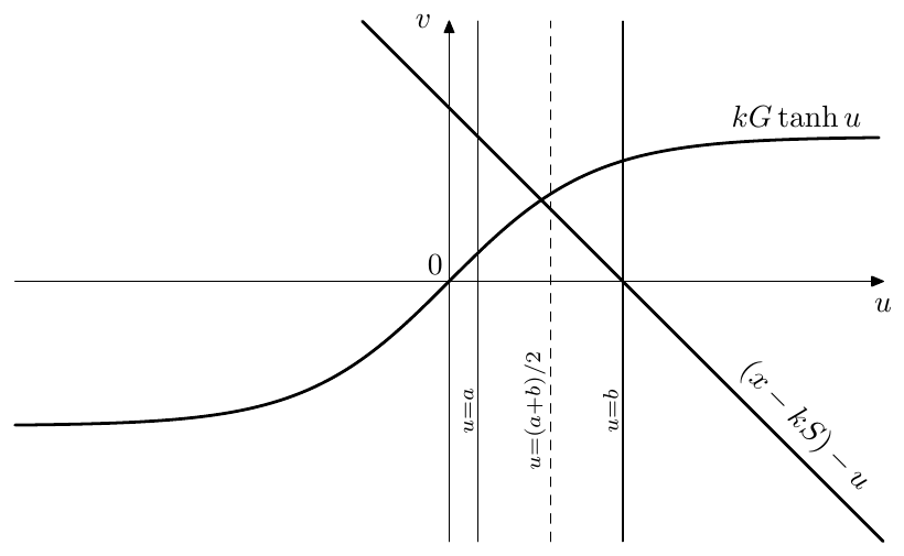
Figure 6.21: Bisection method.
Obviously the size of the bracketing range halves on each step and we repeat the procedure until the bracketing range becomes sufficiently small. The convergence speed therefore doesn’t depend on values of filter’s parameters or signals and the iteration is guaranteed to converge. However we need to be able to somehow find the initial bracketing range .
Fortunately, with monotonic saturation shapes such as this is not very difficult. We can construct the initial bracketing range by noticing that the graph of the function lies between and (Fig. 6.22).
With unbounded saturators such as inverse hyperbolic sine one needs to get slightly more inventive. One possible idea is shown in Fig. 6.23. This however doesn’t work for . In that case we could reuse the approach of Fig. 6.22 by taking a vertically offset version of (6.5) as a bound on (Fig. 6.24). The intersection on with this bound can be found by solving a quadratic equation (more on this in Section 6.7). Obviously, the same idea works for too.
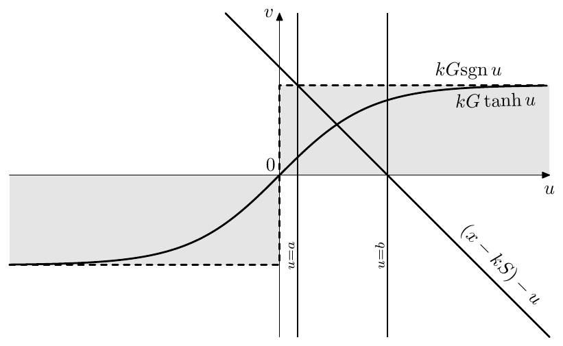
Figure 6.22: Initial bracketing for bisection.
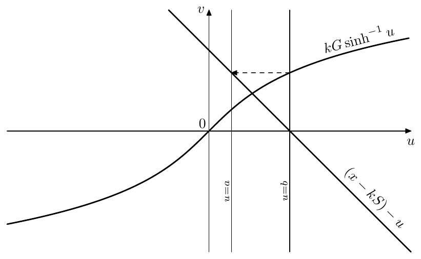
Figure 6.23: Initial bracketing for bisection in the case of an unbounded saturator and . First we find the right bracket and then use to find the left bracket .
If nothing else helps to find the initial bracketing range for a (monotonic) nonlinearity , one could simply start at some point, such as e.g. the zero-crossing of , determine the direction of other bracket by comparing to and then take steps of progressively increasing size (exponential increasing of steps is usually a good idea) until the comparison result of and flips.
Even though bisection method guarantees convergence, the convergence speed might be a bit too low for our purposes. Let’s assume that the magnitude order of the signals in the filter is and let’s assume that the length of the initial bracketing segment has about the same order of magnitude. Then, to reach a dB SNR14 corresponding to the order of magnitude of , we’ll need about 10 iterations. This might be a bit too expensive for a realtime audio processing algorithm on modern computers.15
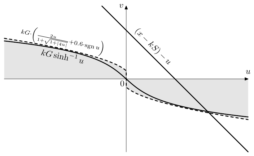
Figure 6.24: Initial bracketing for bisection in the case of and .
6.6 Approximate methods
We might also attempt to find a rough approximate solution of (6.12) without running an iterative scheme. Having found , we would simply pretend it’s a true solution, and proceed as usual in the zero-delay feedback solution scheme, sending through the tanh waveshaper and further through the 1-pole lowpasses, updating their state along the way. Several approximation approaches seem to be in (more or less) common use:
Linearization at zero
At small signal levels the nonlinearity is almost transparent:
Hoping that our signal level is “sufficiently small”, whatever that means, we could replace by and solve the resulting linear equation:
Note that this is equivalent to one step of Newton-Raphson with as the initial guess.
Linearization at operating point
Hoping that the signals within the filter do not change much during one sample tick, we replace with its tangent line at the current point:
where is the value of at the previous discrete time moment. This is equivalent to one step of Newton-Raphson with as the initial guess. Usually this approximation provides a better result, however in the excessive (but not so unusual) situations of high cutoff, high feedback amount and/or high signal frequencies this can work worse than the linearization at zero. Thus, the linearization at zero might provide a better “worst case performance”.
Linearization by secant line16
On the graph of we draw a straight line going through the origin and the operating point and use this line as our linearization to obtain the value of . Being a mixture of the previous two approaches, in moderately excessive situations this could work better than the linearization at the operating point, but at more excessive settings could work worse than the linearization at zero. The readers are however encouraged to gain their own experience and judgement in the choice of the initial guess approach.
All the above quick approximation approaches share the same idea of replacing the nonlinearity with a straight line. In that regard it is important that we have chosen to solve for the signal at the saturator’s input, so that the signal obtained through the approximation is then really sent through the nonlinearity before reaching the 1-poles and the output. One can view this as if, after having obtained the approximated result, we are doing one step of fixed-point iteration.17 Had we instead chosen to solve for the signal at the saturator’s output, the results would have been more questinable. Particularly, in the case of linearization at zero there would have been no difference to the linear case whatsoever.
The above approximation approaches work reasonably well with saturation type of nonlinearities. Obviously, the error increases as becomes larger and thus the system becomes “more non-linear”. Notably, , being monotonically growing in respect to , decreases as the sampling rate grows, thus the approximation error is smaller at higher sampling rates.
6.7 2nd-order saturation curves
It is possible to avoid the need of solving the transcendental equation by using a saturator function which still allows analytic solution. This is particularly the case with second-order curves, such as hyperbolas. E.g. can be replaced by (which consists of two hyperbolic segments), thereby turning (6.13) into:
The inverse of can be replaced by the inverse of , consisting of two parabolic segments.
In order to solve (6.18), which graphically is an itersection between the lines and (same as in Figs. 6.13, 6.14, 6.15), we first need to find out, whether the intersection is occuring at or (the case can be included into either of the cases). Looking at Figs. 6.13 and 6.14, it’s not difficult to realize that for this is defined solely by the sign of the value which takes at . Thus (6.18) turns into
Each of the equations (6.19) is a quadratic equation in respect to .
Choosing the appropriate one of the two solutions of the quadratic equation is easy. E.g. for (6.19a) the choice can be made with the help of Fig. 6.25. Taking into account the restriction , we see that we should be alway interested in the larger of the two solutions , . The choice of the appropriate solution for (6.19b) can be done using similar considerations.
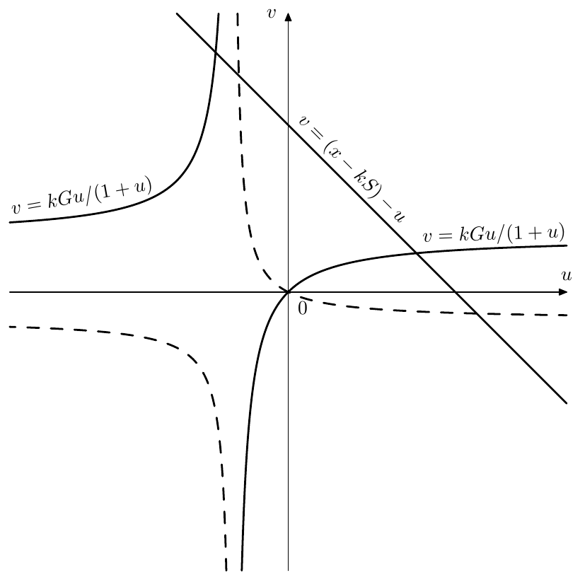
Figure 6.25: Choice of the solution of the quadratic equation for . The dashed line shows the graph of for .
In solving the quadratic equation one has not only to choose the appropriate one of the two roots of the equation, but also to choose the appropriate one of the two solution formulas:
Mathematically the two formulas are equivalent, however numerically there is a precision loss (which may become very strong) if results in addition of two values of opposite sign, or, conversely, subtraction of two values of the same sign. This consideration yields the following formulas for the solutions of the quadratic equation:
2nd-order soft clippers of the most general form
We could generalize the previously used idea of turning the nonlinear zero-delay feedback equation into a quadratic one by considering a waveshaper made of the most general form of a second-order curve defined by18
Equation (6.21) has 6 parameters and 5 degress of freedom. After subtituting the nonlinearity (6.21) into (6.13), the equation (6.13) turns into
or, equivalently,
Obviously, (6.22) is a quadratic equation in respect to . Particularly, under the “typical soft clipping curve” conditions
equation (6.21) turns into a family of hyperbolas: with a single parameter:
Four of five freedom degrees in (6.21) has been taken by the conditions (6.23). The fifth remaining degree is represented by the parameter , which is the value19 of that the curve has at (Fig. 6.26). A reasonable choice for the range of is , where at we obtain the already familiar curve, at the curve (6.24) turns into a hardclipper.
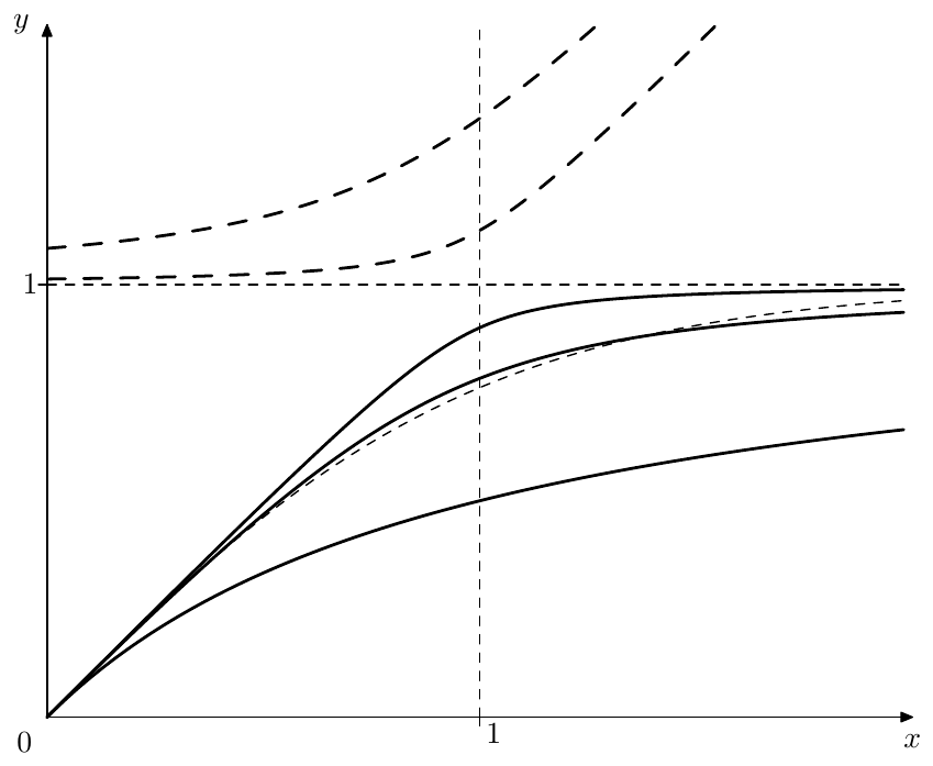
Figure 6.26: A family of soft clippers generated by (6.24) for , and . The two dashed curves above the line are the second (unused) branches of the respective curves (the second branch for is not visible because it is outside the picture boundaries). The thin dashed curve close to the main branch of the curve for is the hyperbolic tangent .
By making the odd extension of the curve:
we obtain a proper soft clipping saturator shape, where we should remember to pick the appropriate branch of the curve, when solving the quadratic zero-delay feedback equation (6.22).
This time the selection of the appropriate solution of the quadratic equation is still simple for , where we can just pick the larger of the two solutions , , however for it becomes more complicated (Fig. 6.27). From Fig. 6.27 one can see that our choice of the larger or smaller of the two solutions is switched once when changes sign and once again when the oblique asymptote of 20 goes at , thereby becoming parallel to to the line .21
By writing out the expressions for the solutions of the resulting quadratic equation, one could see that, if we define the choice of the solution in terms of the choice of the plus or minus sign in (6.20) in front of (which is actually what we care about), then the solution is switched only when , at which moment and respectively both solutions become equal to each other. The (negative) value of , at which the oblique asymptote of goes at , doesn’t correspond to another solution switch but solely to the unused solution disappearing into the infinity from one side and reappering from the other.
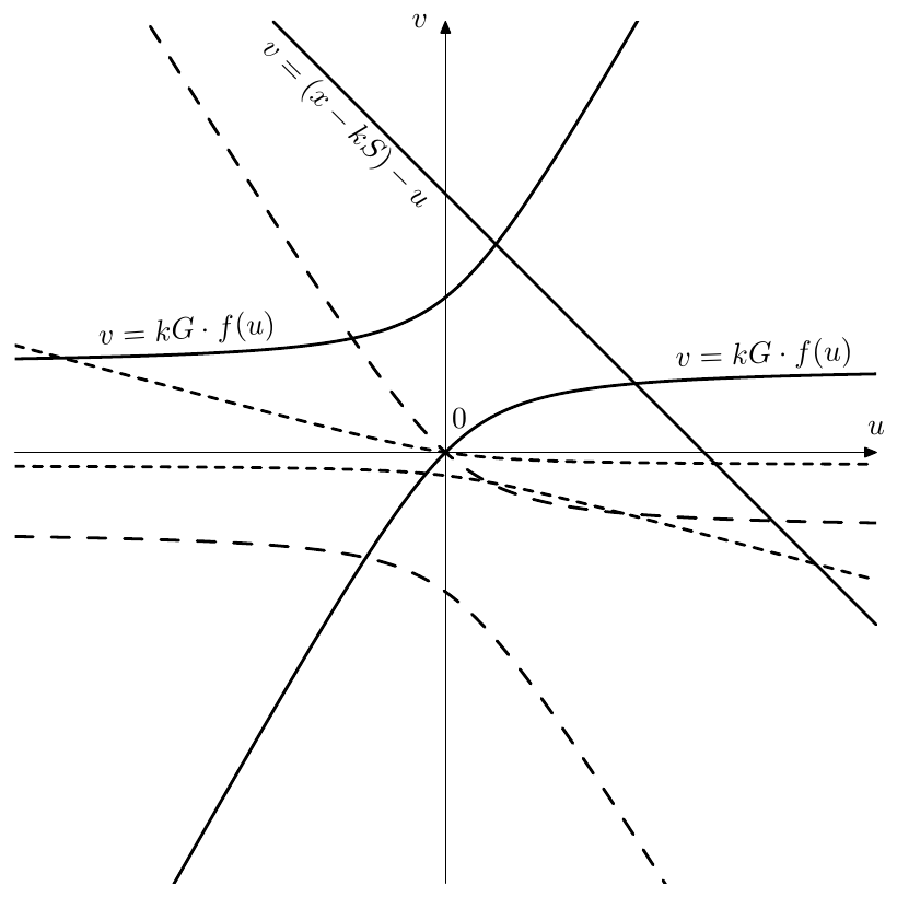
Figure 6.27: Choice of the solution of the quadratic equation for which is a member of the family of hyperbolas (6.24). Solid line corresponds to , dashed lines correspond to two different values of .
Other 2nd-order saturators
Apparently, mixing in a linear component (6.6) into a saturator defined by (6.21) still can be expressed in the general form (6.21), thus the zero-delay feedback equation is still quadratic equation and we can use the same solution techniques.
Instead of using hyperbolas, we could also use parabolas, such as the one in (6.5) or its mixture with a linear term. Ellipses, having finite support in terms of both and , are not lending themselves for this kind of usage, unless used in a piecewise approximation, which we discuss later.
6.8 Tabulation
Tabulation is one of the standard ways of reducing the computation cost of functions. Instead of computing the function using some numerical method (which might be too expensive) we store function values at certain points in a lookup table. To compute the function value in between the points, interpolation (most commonly linear) is used.
Tabulation is worth a dedicated discussion in the context of nonlinear zero-delay feedback equations, because in this case it can be combined with the bisection method in a special way, making this combination more efficient. Also the same ideas provide a general framework for applying piecewise saturation curves in a zero-delay feedback context, even if the number of segments is so low that using a real table is not practical.
Imagine the saturator function in Fig. 6.13 was represented by tabulation combined with linear interpolation, which effectively means that we are having a piecewise-linear function (Fig. 6.28). In order to solve (6.13) we first would need to determine the applicable segment of . Having found the linear segment we just need to solve a linear zero-delay equation.
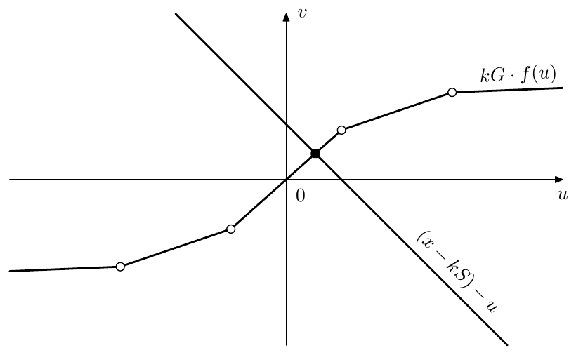
Figure 6.28: The solution of (6.13) for a piecewise-linear saturator.
From Fig. 6.28 is should be clear that the bisection method for a piecewise-linear curve can be implemented by simply comparing the values of and at the breakpoints , thereby sparing the need for linear interpolation. We would start with some initial bracketing of the breakpoint range and then compare the two curves at the breakpoint in the middle of the range (where , rounding the result of division by 2 up or down, if necessary). Depending on the comparison outcome we pick either or as the next range. We repeat until we are left with a single segment, and then simply solve the linear zero-delay feedback equation.22
The very first and very last linear segments will require special care, because they do not go from one table point to the other, but extend from the outermost entries of the table to . We can either assume that they horizontally extend from the first and last points in the table, or store their slope separately.
As a very simple example of the just introduced concepts we could consider a hard clipper
(Fig. 6.29). We don’t need a real table to store the breakpoints, but the same ideas apply. First comparing and at we find out whether the intersection occurs in the right-hand saturation segment . If not, then we perform the same comparison at , thereby finding out whether the intersection occurs in the left-hand saturation segment . Otherwise the interesection occurs in the middle segment .23
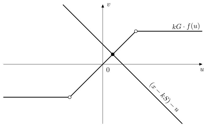
Figure 6.29: The solution of (6.13) for a hard clipper.
The tabulation approach is not limited to piecewise-linear segments. We could e.g. use the 2nd-order segments of the form (6.21). Since the latter have 5 degrees of freedom, we could use 4 of those to specify the values of the function and its first derivative at the segments ends (like we would do for a Hermitian interpolating segment and like we did for (6.24)) and use the 5th degree of freedom e.g. to minimize the remaining error. In fact, in Section 6.7 we have done exactly this, building a piecewise-2nd-order curve consisting of two segments joined at the breakpoint at the origin. The saturator (6.2b), consisting of four segments of an order not exceeding 2, could be another candidate for this approach.
6.9 Saturation in 1-pole filters
The feedback in the 1-pole filter is not one creating the resonance. Therefore the discussion from Section 6.3 does not apply and we need to address nonlinear 1-poles separately.
We are going now to discuss nonlinear 1-poles with the nonlinearity ideas derived from different analog variations of the 4-pole lowpass ladder filter discussed in Section 5.1 These nonlinear 1-pole filters, however, are of generic nature and are therefore not limited to the usage inside 4-pole lowpass ladder filters (or inside filters of whatever specific kind, for that matter).
Transistor ladder’s 1-pole lowpasses
The linear model of transistor ladder discussed in Section 5.1 (Fig. 5.1) is a first level of approximation of the behavior of the respective analog structure, where we ignore all nonlinear effects. If we wish to take nonlinear effects into account, we could replace the underlying linear 1-pole lowpasses of the ladder filter with nonlinear 1-pole lowpasses, the structure of such nonlinear lowpass being shown in Fig. 6.30. In terms of the equations, (2.3) is transformed into
The lowpass in (6.25) and Fig. 6.30 is a simple nonlinear model of the underlying 1-pole lowpass of the transistor ladder, directly arising out of the application of Ebers-Moll transistor model.24
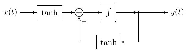
Figure 6.30: A nonlinear 1-pole lowpass element of the transistor ladder filter.
Which effect does the change from (2.3) to (6.25) have? Apparently, has a smaller absolute magnitude compared to , the drop in magnitude becoming more noticeable of one or both of the signals and is sufficiently high. If both and have large values of the same sign, it’s possible that the difference is close to zero, even though the difference is very large. This means that the filter will update its state more slowly than in (2.3). Intuitively this feels like “cutoff reduction” at large signal levels, or, more precisely this can be seen as audio-rate modulation of the cutoff, where the cutoff is being changed by the factor
where the equality is attained at .
Connecting 1-poles from Fig. 6.30 in series (Fig. 6.31) can be optimized by noticing that we don’t need to compute the tanh of the output of the first integrator twice (Fig. 6.32), thus sparing one tanh saturator. The entire ladder filter thereby turns into one in Fig. 6.33.

Figure 6.31: Serial connection of two nonlinear 1-pole lowpass el- ements from Fig. 6.30.
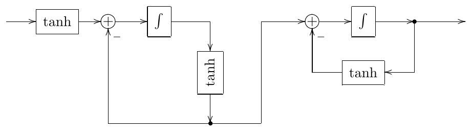
Figure 6.32: Optimized serial connection of two nonlinear 1-pole lowpass elements from Fig. 6.31.
The nonlinear 1-pole in Fig. 6.33 are normally sufficient to prevent the filter from explosion in selfoscillation range. However, obviously, there is nothing which should stop us from introducing additional nonlinearities, such as the ones discussed in Section 6.3, not so much as a means from preventing the filter explosion but rather for giving additional color to the sound. Apparently feedfoward path of Fig. 6.33 already contains many nonlinear elements, therefore adding nonlinearities to the feedback path could make more sense. Note that while there are good reasons to keep the saturation levels of nonlinearities in the feedfoward path of Fig. 6.33 (especially since we are employing the optimization from Fig. 6.32, which shares one nonlinearity between two 1-pole lowpasses), there is much less reason to have the same saturation level (or even the same saturation curve) for the nonlinearity in the main feedback path.
The nonlinear version of the diode ladder filter (Figs. 5.48, 5.49) is using a similar kind of nonlinear 1-poles, resulting in a structure shown in Fig. 6.34.
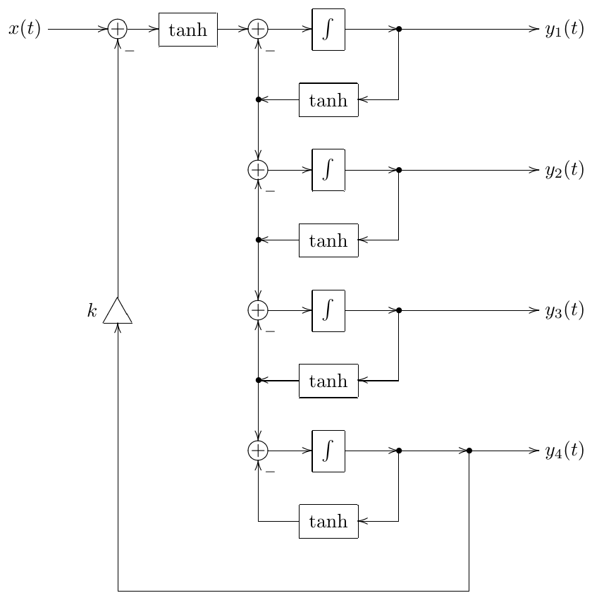
Figure 6.33: Nonlinear transistor ladder filter.
The equations (5.18) are respectively turned into:
(compare to (6.25)).
OTA ladder 1-poles
The same idea of the ladder filter discussed in Section 5.1 and shown in Fig. 5.1 has been often implemented in analog form using OTA (operational transconductance amplifiers) instead of transistors. This generates another kind of nonlinear 1-pole structure (Fig. 6.35).
Formally we are having a feedback loop saturator here. However this feedback loop is not responsible for generating the resonance, therefore the effect of the saturator is different from the one discussed in Section 6.3. We are having a saturator at the integrator’s input, therefore we are performing soft clipping on the speed of change of the filter’s output value, or, equivalently, we are doing “soft slew limiting”. Alternatively, as shown by (6.8), this can be seen as audio-rate cutoff modulation, the cutoff factor varying in agreement with (6.9).
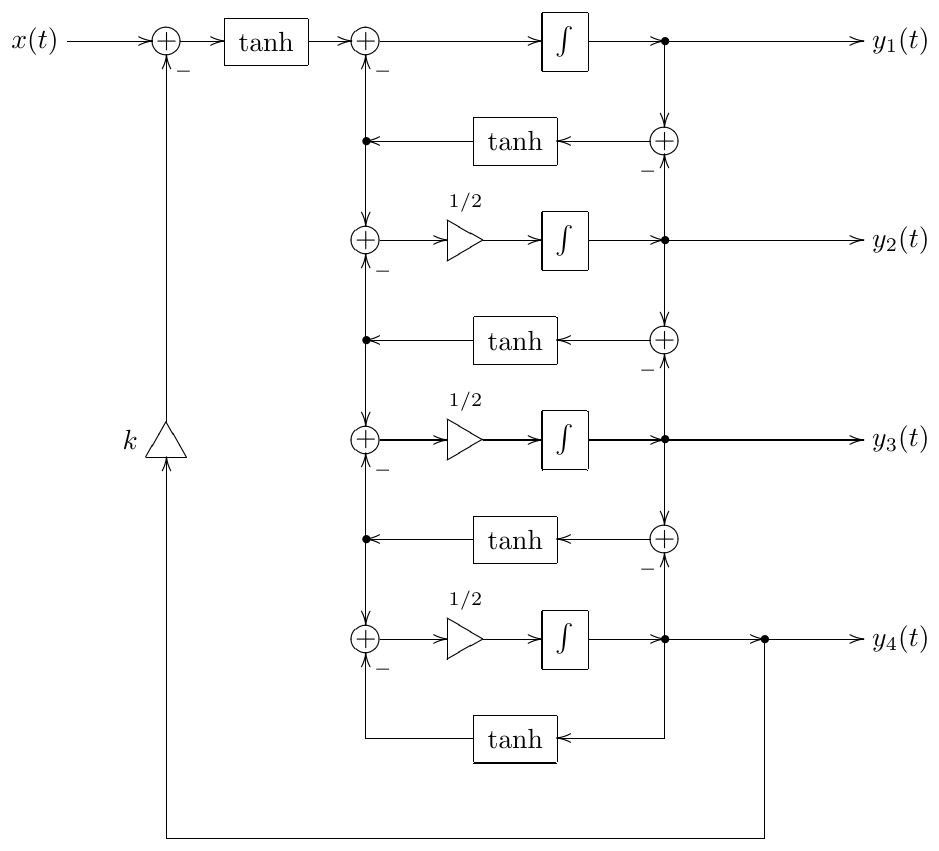
Figure 6.34: Nonlinear diode ladder filter.
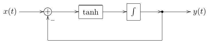
Figure 6.35: OTA-style nonlinear 1-pole lowpass.
Note that we have two different options for picking the highpass signal in Fig. 6.35. We could do this either before or after the nonlinearity. In the latter case the highpass signal will be saturated (which might be a bit over the top, compared to the lowpass signal), in the former case we have the benefit of preserving the relationship . This also makes the former option look like a particulary good candidate not only for a nonlinear 1-pole highpass (and thereby, among other things, for ladder filter structures utilising highpasses) but also for a nonlinear allpass. Fig. 6.36 shows the respective nonlinear 1-pole multimode.
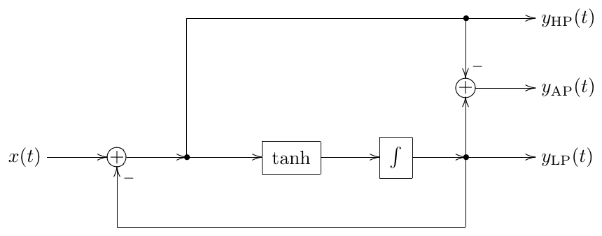
Figure 6.36: OTA-style nonlinear 1-pole multimode.
Saturated integration
The previously discussed ways of introduction of nonlinearities into 1-poles resulted in relatively complicated nonlinear behavior of the filters. But what if we want a simpler behavior? Let’s say we want to simply saturate the output. Of course we simply could put a saturator at the output of the filter (Fig. 6.37) but this doesn’t really feel like making the filter itself nonlinear.
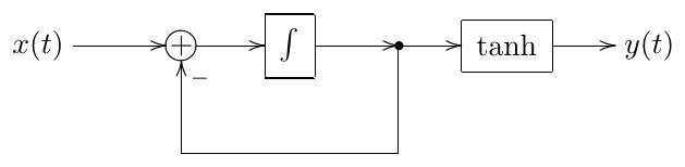
Figure 6.37: Putting a saturator at the filter’s output.
We could try putting the output nonlinearity inside the filter’s feedback loop (Fig. 6.38). However, comparing this to equation (2.3) we should realize that the main effect of such nonlinearity will be that the difference will be changed to , leading to the capacitor in Fig. 2.1 continuing to charge even after the output value has reached the input value. In other words, the output will still grow even after reaching the input value. This feels more like a mistake.
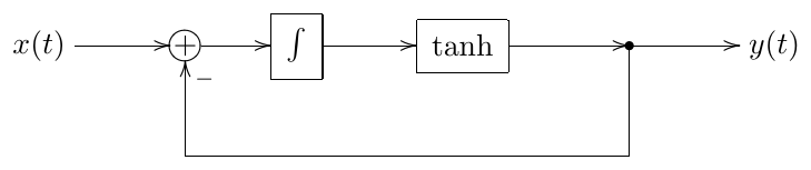
Figure 6.38: Saturating the integrator’s output (not really a working idea).
What we rather want is to prevent the 1-pole’s capacitor in Fig. 2.1 from charging beyond a certain level (that is we want to prevent the integrator state from going beyond a certain maximum). In order to achieve that in a “proper analog way”, we will need to introduce antisaturators, which we are going to do later in this chapter. However we could also do a “hack” and modify the integrator structure, introducing the saturation into its internal accumulation process. This works particularly well with direct form I (Fig. 6.39) and transposed direct form II (Fig. 6.40) integrators. Obviously, this hack is not limited to 1-poles, but can be applied to any structure which is based on integrators, such as e.g. SVF.
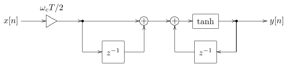
Figure 6.39: Saturating direct form I trapezoidal integrator.
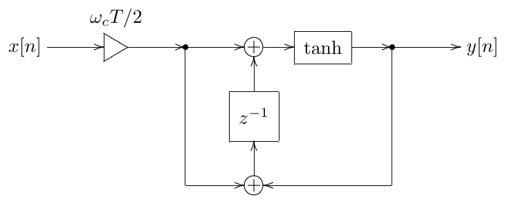
Figure 6.40: Saturating transposed direct form II trapezoidal integrator.
6.10 Multinonlinear feedback
We have seen that instantaneous responses of linear filters are linear functions of their input, such as e.g. in (3.29). It is not difficult to realize, particularly from the previous discussion of the solution of the nonlinear zero-delay feedback equation (6.12), that instantaneous response of a nonlinear filter is some nonlinear function of its input:
(where we also explicitly notated the dependency on the filter’s state , but the dependency of on the filter’s parameters is understood implicitly).
Consider the OTA-style 1-pole lowpass in Fig. 6.35 and imagine we build a 4-pole lowpass ladder filter (as in Fig. 5.1) from four idenitical 1-pole lowpasses of this kind. Assuming (6.26) decribes the instantaneous response of Fig. 6.35, we could redraw Fig. 5.1 in the instantaneous response form as Fig. 6.41.

Figure 6.41: Nonlinear ladder filter in the instantaneous response form.
Let denote the signal at the input of the first 1-pole lowpass in Fig. 6.41. The zero-delay feedback equation for the entire of Fig. 6.41 therefore becomes
Intuitively we can expect to be monotonically increasing with respect to , thus should be monotonically increasing too, and we could use most of the previously described methods of solving nonlinear zero-delay feedback equations to solve (6.27). Theoretically.
Practically the evaluation of is usually very expensive, because it means a numerical solution of the zero-delay feedback equation for the respective 1-pole, possibly running several rounds of an iterative method. Now, if we are going to use an iterative method to solve (6.27), these expenses will be multiplied by the number of the “outer” iterations. Besides, if we are using Newton-Raphson to solve (6.27) then we need not only to evaluate but also its derivative with respect to , which further increases the computation cost of solving (6.27).
Therefore usually such “nesting” approach, where we express the higher-level zero-delay feedback equation in terms of the solutions of the lower-level zero-delay feedback equations, is not very practical for nonlinear systems. Instead, let’s “flatten” the entire structure, and write the equation describing the instantaneous response signals within this structure. E.g. for the 4-pole ladder built out of 1-poles in Fig. 6.35 the flattened structure is shown in Fig. 6.42. Or, representing the integrators by their instantaneous responses (which are fully linear), we obtain Fig. 6.43.
Denoting the input and output signals of each of the 1-poles as and , we write the 1-pole zero-delay feedback equations:
Or, since we can denote the input of the first lowpass as and write
Plus, we are having the global feedback loop:
and thus we are having an equation system:
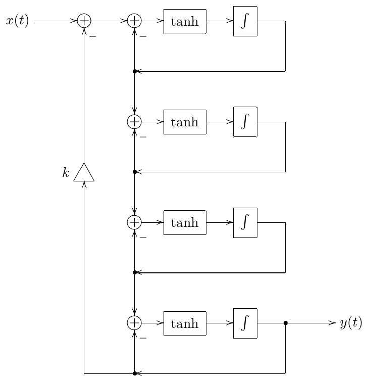
Figure 6.42: Flattened OTA lowpass ladder filter structure.
We can get rid of the first equation by simply substituting its right-hand side for , obtaining:
Equation (6.28) can be written in a more concise form by introducing the vector
and the vector-function of a vector argument :
In this notation (6.28) looks simply like
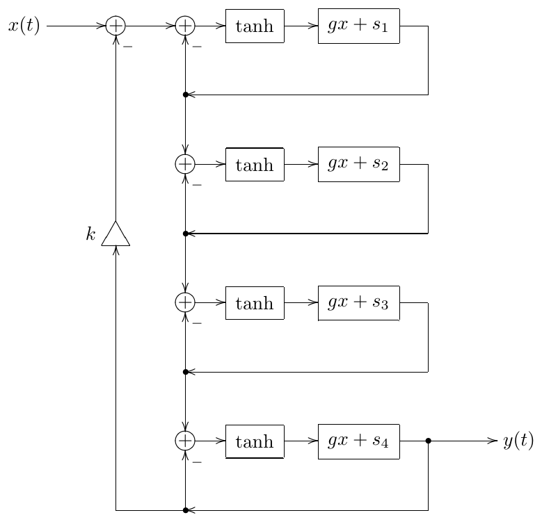
Figure 6.43: Flattened OTA lowpass ladder filter structure in the instantaneous response form.
This is our nonlinear 4-dimensional (since we are having 4 unknowns ) zero-delay feedback equation.
The form (6.29) readily offers itself for fixed-point iteration. By rewriting (6.29) as
the multidimensional form of Newton-Raphson algorithm can be used:
Also the quick approximate methods of Section 6.6 work out of the box.
The difference of solving (6.29) instead of (6.27) is that in (6.29) we are simultaneously solving all zero-delay feedback equations in the system, thereby not having the problem of nested iterations.
Actually, choosing the 1-pole output signals as the unknowns is not necessarily the best choice. It would have been more convenient to solve for the inputs of the integrators, so that we can directly reuse the obtained signals to update the integrator states.25 On the other hand, e.g. for the transposed direct form II integrator (Fig. 3.11) one could deduce the new state from the old state and the new output signal, thus also work pretty efficiently (this trick has been used in the digital implementation of an SVF in Section 4.4). A consideration of a bigger importance therefore could be that the choice of the unknowns may affect the convergence of the iteration scheme.
Usually for multidimensional zero-delay feedback cases the iterative methods need to be further refined and/or a combination of different methods need to be used to have a reliable and quick convergence of an iterative process of finding the solution of (6.29). However, often simply using the approximate methods of Section 6.6, will deliver reasonable results.
6.11 Antisaturators
In Section 6.9 we made some attempts to make the 1-pole lowpass filter state saturate, the most successful attempt being the modification of the internals of an integrator. In a real analog circuit we wouldn’t have been able to do the same, as e.g. a capacitor, which is used as an integrator for the current, doesn’t have “built-in saturation functionality”. Therefore different means have to be used to achieve the integrator state’s saturation.
Diode clipper
A common trick is to shorten the 1-pole filter’s capacitor with a nonlinear resistance, this resistance being high at low voltages and dropping down at high voltages on the capacitor. That is the short path is disabled at low voltages but progressively “turns on” at higher voltages. This can be done by using a diode pair (Fig. 6.44). The structure in Fig. 6.44 is commonly referred to as diode clipper.
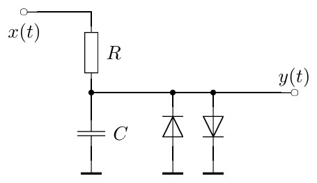
Figure 6.44: Diode clipper.
Using Shockley diode equation we can show that, qualitatively, the current flowing through the diode pair is related to the capacitor voltage as
where and are diode parameters (Fig. 6.45 provides a graph of sinh as a reference). This current is then subtracted from the current which is charging the capacitor, thus acting as current leakage:
(please refer to equations (2.1) for the other details of the circuit’s model). Since is very small, as long as is below or comparable to the leakage is negligible. As exceeds , the current grows exponentially and quickly stops being negligible.
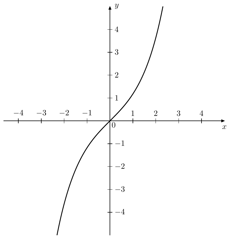
Figure 6.45: Hyperbolic sine .
In terms of the block diagram (Fig. 2.2) this current leakage can be expressed as shown in Fig. 6.46, where we have assumed that the filter cutoff is controlled by the resitance rather than capacitance and thus the amount of the current leakage is independent of the cutoff.
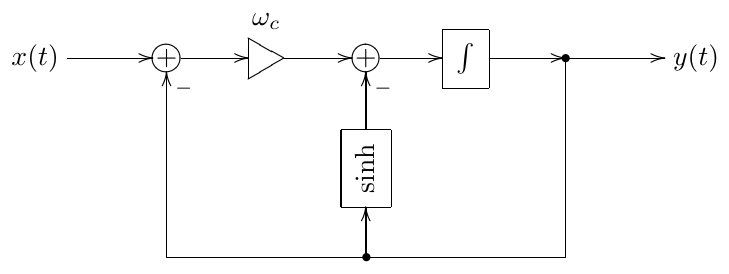
Figure 6.46: Diode clipper in the form of a block diagram. “sinh” stands for some curve of the form “”.
The fact that the leakage current is independent of the cutoff is actually having the opposite effect: the effects of the leakage become cutoff-dependent and the leakage more strongly affects the filter at lower cutoffs. Particularly, given a constant input voltage, the stabilized output level will be larger at larger cutoffs. For the purposes of generic application it is therefore more useful to make the leakage cutoff-independent, as in Fig. 6.47.
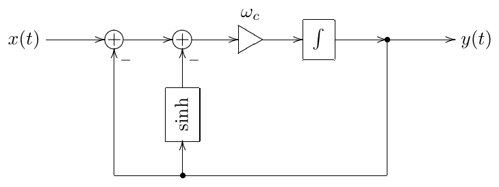
Figure 6.47: Diode clipper with cutoff-independent leakage. “sinh” stands for some curve of the form “”.
Or, using implied cutoff notation and combining the two feedback paths into a single one, we obtain the structure Fig. 6.48. Also, in Fig. 6.47 the cutoff parameter was not the true cutoff of the system, since at low signal levels the gain of the feedback path was . This made the system behave as if its cutoff was and as if its input signal was reduced by factor at the same time. In Fig. 6.48 we addressed this issue by scaling the linear path of the feedback by the factor . This doesn’t change the qualitative behavior of the system, but affects only the interpretation of the cutoff and the input signal scale.
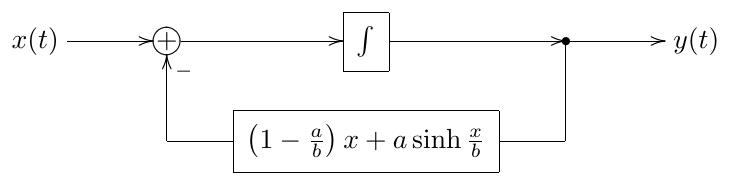
Figure 6.48: Diode clipper with cutoff-independent leakage (simplified diagram).
The structure in Fig. 6.48 is a good illustration of the idea that we could employ to introduce saturation into 1-pole lowpass filter’s state: as grows exponentially for large signals, the term causes the negative feedback to grow as well, thereby causing the integrator to “discharge”.
The same effect is obviously obtained by putting any other quickly growing function of a similar shape into the feedback path of a 1-pole lowpass. Good options for such functions are provided by the inverses of the saturator functions introduced in Section 6.2:
A particularly important feature of the inverses of the saturators is that, same as with saturators, they are transparent at low signal levels, thereby not affecting the cutoff of the filter.
We will refer to the waveshapers having an inverse saturator kind of shape as antisaturators. Fig. 6.49 shows another version of Fig. 6.48, this time using a simpler antisaturator.
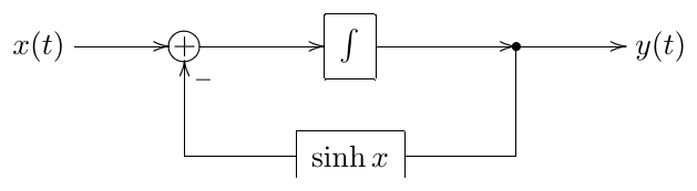
Figure 6.49: Lowpass filter’s state saturation by using an antisaturator.
An antisaturator in Fig. 6.49 is having a similar effect on the filter’s state saturation as its inverse (the respective saturator) would have had if directly applied to a signal, or if being put in a resonating feedback path. Specifically, using an unbounded saturator’s inverse as an antisaturator in Fig. 6.49 would result in an unbounded saturation of the filter’s state, in the sense that by making the amplitude of the input signal of the filter larger and larger one can achieve arbitrarily large levels of the filter’s state. On the other hand, using a bounded saturator’s inverse as an antisaturator (such as e.g. ) would result in bounding of the filter state, the state not being able to exceed the saturation level.
As with saturators, adding a linear term to an antisaturator doesn’t change its antisaturating behavior, but simply weakens it a bit further, where we assume that the addition should be done under the same considerations of keeping the transparency at low signal levels:
The antisaturator in Fig. 6.48 is a kind of a reverse example of this principle, which can be seen as if the (otherwise fully linear and transparent) shape was modified by an addition of a non-transparent antisaturator , however the resulting curve has been made transparent again.
Antisaturation in SVF
As with 1-pole filters, the feedback in SVF is also not one creating the resonance, respectively the discussion from Section 6.3 does not apply either, and thus we can’t simply put a saturator into the feedback loop. Actually, the purpose of the feedback in SVF is kind of an opposite of creating the resonance. The function of the feedback path containing the bandpass signal is to dampen the otherwise self-oscillating structure. This suggests the idea that if we put an antisaturator into the bandpass signal path, this might actually do the trick of preventing the signal levels from getting too high.
Our first attempt to do so is shown in Fig. 6.50. After thinking a bit we, however, realize that it can’t work. Indeed, at there is no damping signal whatsoever, the same as without the antisaturator. Furthermore, probably the main reason to introduce the antisaturator into the SVF is so that we could go into the selfoscillation range , same as we did e.g. with nonlinear 4-pole ladder by going into the range . However, at the introduced antisaturator doesn’t cause any damping either, quite on the opposite, it amplifies the “antidamping” (the inverted damping signal). Obviously, putting the antisaturator after the gain element instead of putting it before doesn’t change much in this regard.
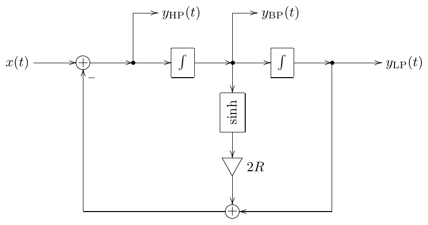
Figure 6.50: An attempt to introduce an antisaturator into an SVF (not really working).
We could get a bit smarter and connect a saturator in parallel with the gain element (Fig. 6.51). This now does the job of saturating the signals, as the damping feedback signal will grow exponentially at large levels of , no matter what the value of is. However now the effective gain of the damping feedback path (at low signal levels, where ) is , rather than .
The latter problem is fixed in Fig. 6.52. In this structure, at the neutral setting of the entire damping signal goes through the antisaturator. This exactly matches the same situation in our first attempt in Fig. 6.50 (and is the reason for the separation of the multiplication by 2 into an additional gain element). As gets away from 1, we send some of the damping signal through the parallel linear path, still keeping the total gain of the damping path equal to at low signal levels.
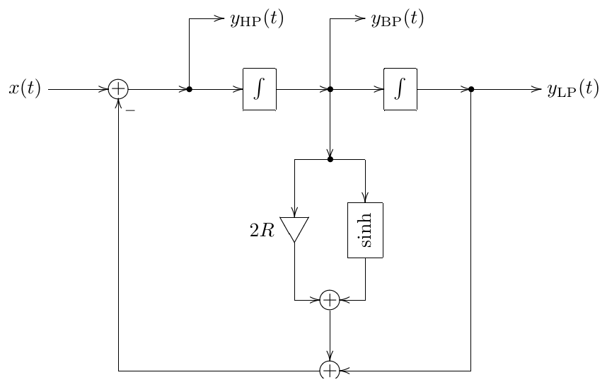
Figure 6.51: A second attempt to introduce an antisaturator into an SVF (works better, but does no longer directly correspond to damping).
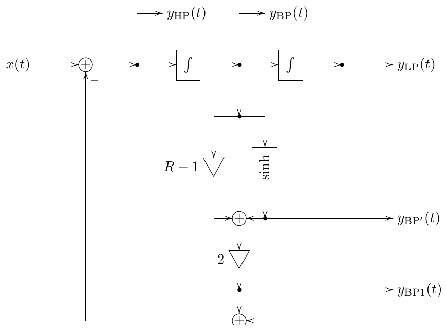
Figure 6.52: An SVF with antisaturator.
The antisaturator in Fig. 6.52 effectively makes the state of the first integrator saturate. This might result in the feeling that the level of the bandpass signal becomes too low. Therefore, instead one could pick the bandpass signal from output, where the antisaturator has increased the level of back. The output provides the normalized bandpass signal.
Note that , as for the linear SVF.
Zero-delay feedback equation with antisaturators
The introduction of antisaturators raises some new considerations for the solution of the zero-delay feedback equation. We will use the nonlinear 1-pole in Fig. 6.49 as a demonstration example, however it will also be more instructive to consider an inverse hyperbolic tangent (Fig. 6.53) instead of a hyperbolic sine as an antisaturator.
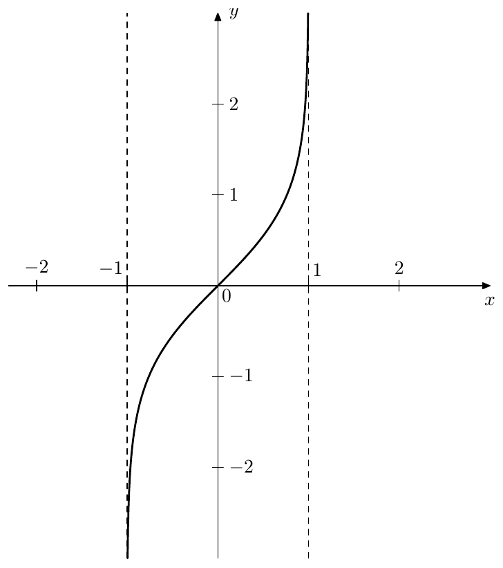
Figure 6.53: Inverse hyperbolic tangent .
Introducing the instantaneous response for the integrator in Fig. 6.49 and replacing with we obtain Fig. 6.54. Writing the zero-delay feedback equation for Fig. 6.54 we obtain
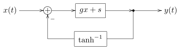
Figure 6.54: Lowpass filter with a antisaturator in the instantaneous response form.
We could start solving (6.30) using the usual methods, such as the ones discussed earlier in this chapter, however notice that has a limited support, being defined only on the range. This might create serious problems if we somehow arrive at a value of outside of that range. Such values of could appear for a number of reasons, such as e.g.:
- from an approximate solution
- from an iterative method’s step
- from numerical errors, such as roundoffs.26
Even if we formally stay within the range , we could still get out of the range of representable values of if gets too large.
There are also related questions of convergence of iterative schemes, particularly of fixed point iteration. Last but not least, close to the boundaries of the range a small numerical error in the value of will result in a huge error in the value of , which suggests that it might be generally a bad idea to explicitly evaluate at all. Similar issues also of course arise with unbounded antisaturators, even though they are not as bad as with bounded ones.
In order to avoid this kind of problems, we can solve for the antisaturator’s output, rather than for the antisaturator’s input. Introducing variable for the antisaturator’s output signal:
we respectively have and can rewrite (6.30) in terms of as
or, further rewriting it so that the linear function in the right-hand side is more explicitly visible
Equation (6.31) looks very much like the previously discussed zero-delay feedback equation (6.13). However, there are still important differences. Expressing the left- and right-hand sides of (6.31) graphically in Figs. 6.55 and 6.56, we see that, compared to Figs. 6.13, 6.14 and 6.15, multiple solutions can occur already for . Fortunately, in Fig. 6.54 the value of cannot get negative, since that would require a negative cutoff value for the integrator.
Having found from (6.31) we can “send” it further through the feedback loop, first finding the integrator’s input value as , then updating the integrator’s state and finding as the output value of the integrator. Note that thereby we never explicitly evaluated .
For an antisaturator in the SVF (Fig. 6.52) the situation is more complicated. We would like to solve for the antisaturator’s output , but then we would be stuck immediately afterwards: since we don’t know the signal on the “” path, we can’t add the output signals from and . Furthermore, we would have a similar problem of not knowing at the next adder (which computes ). These problems are not unexpected, considering that we have been solving for a point in the signal path which is not shared among all zero-delay feedback loops in the structure.
One way around this would be to try to introduce more unknowns into the system and solve several equations at once. However, in this specific case we could simply “send the obtained signal through the antisaturator in the reverse direction”. That is, knowing the antisaturator’s output, we can obtain the antisaturator’s input by evaluating (which is completely okay, we don’t want to explicitly evaluate the antisaturator function because it can increase the computation error by a huge factor, but it is no problem to evaluate its inverse), thereby finding the value of . The signal is shared among all zero-delay feedback loops and therefore is sufficient to find all other signals in the structure.27
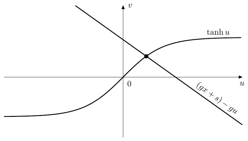
Figure 6.55: The solution of (6.31) for .
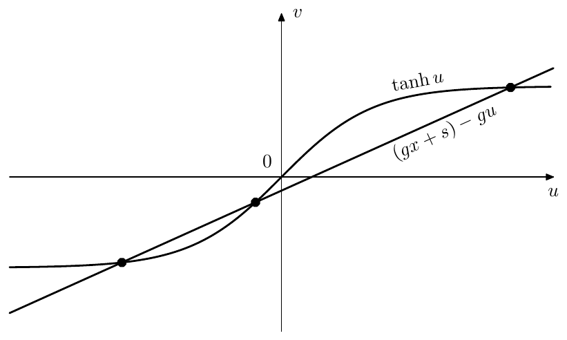
Figure 6.56: The solution of (6.31) for .
The general approach of avoiding the explicit evaluation of antisaturators but rather dealing with their inverses instead also allows us to deal with a certain class of antisaturators which are not functions in the normal sense. An example of this are compact-range monotonic saturators such as (6.2b). The inverse of such saturator is not really a function, since it would have infinitely many different values at (Fig. 6.57). However we still can use it as an antisaturator, since we never have to deal with the antisaturating function explicitly, but are dealing with the respective saturating function instead.28
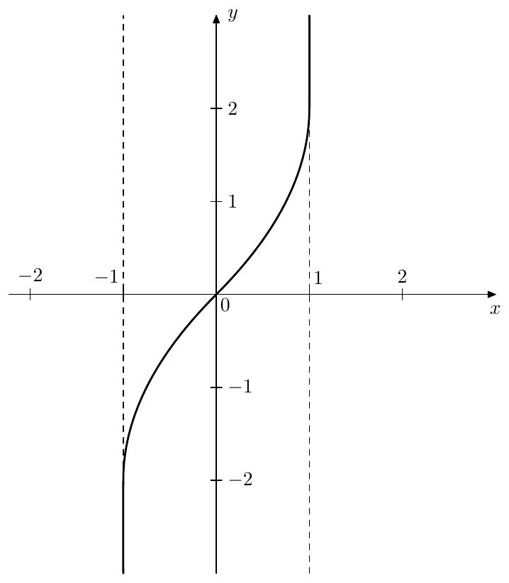
Figure 6.57: The inverse of (6.2b) is not a function in the normal sense.
6.12 Asymmetric saturation
The saturators which we have been using so far were all having the odd symmetry . A feature of all symmetric saturators is that when its input signal amplitude is very high, the output signal basically alternates between positive and negative saturation levels . If the input signal is something like a sine or a sawtooth, the saturator would produce a square-like output. More generally, such saturators tend to produce signals containing mostly odd harmonics (as the square wave does).
Sometimes this domination of odd harmonics can become too boring29 and asymmetric saturation might be desired. Simply adding an offset to the saturator’s input (or, instead, performing a parallel translation of the saturator curve by “sliding” it through the origin, to keep the property ) works only for signals of average levels. At high signal levels the same square would be produced for e.g. a sine or a sawtooth input.
The offset idea would have worked, though, if the offset had been somehow made proportional to the input signal’s amplitude.30 It turns out that this is a natural feature of a particular nonlinear 1-pole construct. Consider the OTA-style nonlinear 1-pole in Fig. 6.36 and imagine that instead of a saturator nonlinearity we have used the following shaper function:
(Fig. 6.58 illustrates). This would mean that whenever , the cutoff is effectively doubled. When , the cutoff is effectively halved. Therefore the integrator state will be more “willing” to change in the positive direction than in the negative one.
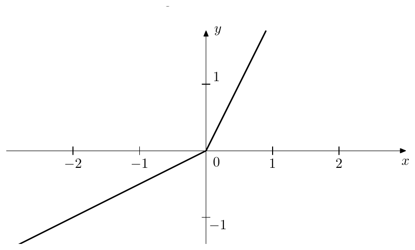
Figure 6.58: “Asymmetric cutoff” nonlinearity.
Imagine such filter receives a steady periodic signal with a zero DC offset (meaning that the average value of the signal is zero, or, in other words, there is an “equal amount” of signal above and below zero). And suppose this signal’s fundamental frequency is well above the nominal cutoff of the filter. In such case a linear lowpass filter would have performed a kind of averaging of the input signal, thereby producing a zero output signal.31 However in the case of using the nonlinearity (6.32) the positive input values will have “more weight” than the negative ones and the lowpass output will be nonzero.
It should be inituitively clear that the lowpass output value will increase as the input signal amplitude increases and vice versa (particularly it should be obvious that in the case of the zero amplitude of the input signal the output signal will also be zero). Therefore, qualitatively such lowpass filter works as an envelope follower, the filter cutoff in a way controlling the envelope follower’s response time. Respectively, the highpass output will contain the input signal with an added (or subtracted) DC offset, such offset being approximately proportional to the input signal’s amplitude. This means that if initially 50% of the signal were above zero and the other 50% below zero, we now have changed this ratio to something like 80% to 20%, and this effect is happening more or less at any amplitude of the input signal.
Thus, asymmetric nonlinear shaping could be produced by the following structure:

where is an initial lowpass, killing the DC offset which might be previously contained in the input signal, is the asymmetric nonlinear highpass, introducing the DC offset into the signal, the signal is then boosted by the gain , controlling the amount of “drive”, and is a usual symmetric saturator.
The nonlinearity (6.32) has a drawback that it contains a discontinuity in the 1st derivative at . Such discontinuity may add a noticeable amount of new harmonic content into the signal. This effect might be desired at times, but for now we would rather at least reduce it, if not avoiding it altogether, as the filter’s main purpose is to introduce the DC offset into the signal. This can be achieved by smoothing the discontinuity. E.g. we could replace (6.32) with a hyperbola going at through the origin, but having a similar to (6.32) asymptotic behavior (Fig. 6.59).
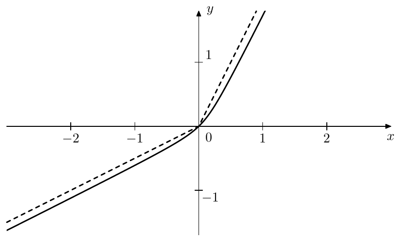
Figure 6.59: Replacing the nonlinearity (6.32) (Fig. 6.58) (dashed line) by a hyperbola.
This kind of nonlinear highpass can occur easily in analog circuits, if nonlinear resistances are involved. E.g. consider Fig. 6.60. The effective resistance connected in series with the capacitor varies, qualitatively speaking, between and a parallel connection of and , depending on the polarity of the voltage over the base-emitter junction of the transistor (where is the emitter-base current ratio). Respectively the cutoff varies (qualitatively) between and . Upon a closer look, the cutoff will vary a bit less than that, because the base-emitter voltage will somewhat reduce the current through , but qualitatively the effect is still there.
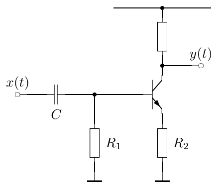
Figure 6.60: Highpass filter with asymmetric cutoff.
6.13 Antialiasing of waveshaping
Aliasing
When a signal goes through a waveshaper, the waveshaping introduces additional partials into the spectrum of the signal. These partials extend into the entire frequency range for almost any waveshaper. We can show that in several steps.
First, let’s consider waveshapers of the form (where ), starting with . Let be a periodic signal. Therefore it can be represented as a sum of its harmonics:
where can be finite or inifinity. Note that we are using complex-form Fourier series, therefore, assuming a real , we have an equal number of positive- and negative-frequency partials. Then
Thus, the frequencies of partials of are all possible sums of frequencies of partials of .32 Respectively the frequencies of the partials of vary between and . That is the width of the spectrum of is twice the width of the spectrum of .
For we obtain
that is the width of the spectrum is tripled. It’s not difficult to generalize it to an arbitrary power of , concluding that increases the width of the spectrum of times.
It should be clear by now that, if is a polynomial of order :
the highest-order term will expand the spectrum of times, while the lower-order terms will also expand the spectrum of but not as much, thus expands the spectrum of times.
Now suppose is a function of a more or less general form, expandable into Taylor series around :
We can consider such as a polynomial of an infinite order and thus expands the spectrum of by an infinite number of times.33
Some of the waveshapers that we were previously discussed were constructed as piecewise functions, including e.g. a piecewise polynomial saturator (6.2b). Would the saturator (6.2b), which consists of polynomial segments of order not higher than 2, thereby expand the spectrum of only 2 times? It turns out that such piecewise function waveshapers also expand the spectrum an infinite number of times. Having discontinuous derivatives themselves (e.g. (6.2b) has a continuous 1st derivative, but three discontinuities of the 2nd derivative), such waveshapers also introduce discontinuous derivatives into their output signal . The presence of discontinuities in a signal’s derivative automatically implies an infinite spectrum of the signal.34
Therefore all waveshapers which we have been considering until now (as well as most of the ones we could even think of) expand the spectrum of the input signal an infinite number of times. This means that discrete-time waveshaping produces aliasing.
Indeed, suppose we are given a waveshaper of a general shape, so that it expands the spectrum of its input signal an infinite number times. And imagine we are having a sampled signal and its corresponding continuous bandlimited version . Assuming unit sampling period we can write . A direct application of a waveshaper to discrete-time signal :
is fully equivalent to sampling the continuous-time signal , by simply letting . However, since expands the spectrum of infinitely, the spectrum of is not bandlimited and simply letting will result in aliased frequencies contained in .
Trying to use polynomial waveshapers doesn’t help much. We could definitely construct polynomial antisaturators, e.g. , whereas a purely polynomial saturator could be constucted only if we know that the input signal has a limited range, which is a pretty heavy restriction. However even will triple the width of the spectrum, so that we’ll need e.g. to bandlimit to one third of the Nyquist frequency, process it by an saturator and add the result to the unprocessed signal:
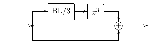
(where BL/3 denotes a filter which bandlimits the signal to 1/3 of the Nyquist frequency, and Lat denotes). Actually bandlimiting will introduce latency into the signal, so we’ll need to add the same latency on the lower path (where Lat denotes a structure which artificially introduces the same latency as introduced by BL/3).
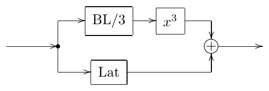
This idea stll doesn’t work really well, since antisaturators are normally used in feedback loops. We can’t perform the bandlimiting inside the feedback loop, e.g.
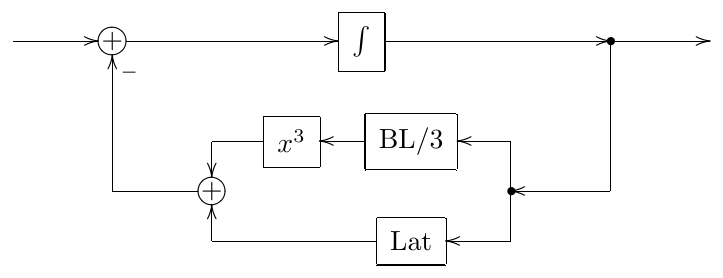
because of the introduced latency. Doing it outside the feedback loop is also problematic. For one, we’d need to bandlimit the entire signal , not only the part of it which goes through the shaper. This still could be done, though, if the sampling rate is sufficiently high (at least ). The other problem is that the signal inside the feedback loop will go infinitely many times through the waveshaper. Therefore bandlimiting of the signal prior to entering the feedback loop to 1/3 of Nyquist frequency won’t really prevent the aliasing from happening.35
Antialiasing
The antialiasing of waveshapers is a difficult problem, not having a universally good solution at the time of writing this text. The only thing which is more or less guaranteed to work is heavy oversampling.36 Unfortuntately, oversampling introduces latency, thus, if e.g. a waveshaper is used in a filter feedback loop, we cannot oversample locally just the waveshaper, but at least the entire feedback loop must be oversampled.
There is however an approach37 which reduces aliasing by a noticeable amount, so that the same quality of sound can be achieved at lower sampling rates than otherwise.38 Suppose we are having a discrete-time signal going through a waveshaper . Instead of sending through the waveshaper in discrete time, thereby producing the discrete time signal
let’s convert to continuous time by means of linear interpolation. Without loss of generality we will consider the linear interpolating segment going between and :
(where we assume unit sampling period ). Applying the waveshaper in contnuous time to this segment we obtain
Now we propose to compute the discrete time sample as
where is some antiderivative of , that is . Or, more generally
where and where is a piecewise linear continuous-time function arising out of linear interpolation of . It might seem that the averaging of on in (6.38) is a somewhat arbitrary operation. However, it isn’t. In fact, such averaging can be considered as one of the simplest possible forms of lowpass filtering the continuous-time signal, aiming to suppress the aliasing frequencies above Nyquist.39
The averaging (6.38) does a reasonable job of reducing the aliasing in compared to (6.35), however it is introducing two problems: latency and ill-conditioning.
Latency
Assuming the transparency of the waveshaper at small signal levels we have and (6.38) turns into
The expression (6.39) describes a discrete time 1-pole lowpass filter with a cutoff at half the Nyquist frequency. Indeed, let’s take the lowpass filter in Fig. 3.31. At (which corresponds to , which in turn corresponds to prewarped half Nyquist frequency ) we have and thus
Combining (6.40b) and (6.40c) we obtain
which is the same as (6.39).
The lowpass filtering effect of (6.38) is actually another problem that we didn’t mention so far. It arises out of the approximations that the method does when converting from discrete-time signal to and back from to . This problem is however not very noticeable at sampling rates of 88.2kHz and higher. So, let’s concentrate on the latency introduced by (6.39).
The averaging in (6.39) can be seen as a mid-way linear interpolation between and and thus intuitively one could expect that it introduces a half-sample delay. This is indeed the case. Taking and assuming , so that the signal’s frequency is far below the cutoff of the lowpass filter (6.39), we have
where since .
It can be shown that the source of this half-sample delay is the averaging of on done in (6.38). Taking where , we have
(where is the cardinal sine function). Thus (6.39) and (6.38) indeed introduce a delay of half sample. Inside a zero-delay feedback loop this would be a serious problem. In order to develop an idea of how to address this problem, let’s look at a few examples.
Waveshaper followed by an integrator
Suppose a waveshaper is immediately preceding an integrator, as shown in Fig. 6.61 (this particularly happens in the OTA-style 1-poles in Figs. 6.35 and 6.36). Normally we recommended to use transposed direct form II integrators however this time we suggest to use a direct form I integrator (Fig. 6.62). Looking at the first half of the direct form I integrator (highlighted by the dashed line in Fig. 6.62) we can notice that it exactly implements the formula (6.39). So, the first part of the integrator implements a half-sample delay too and does so in exactly the same way as the antialiased waveshaper for low-level signals. This therefore leads to an idea to simply drop this part of the integrator, as it is done in Fig. 6.63, since we are getting the same half-delay from the waveshaper already.
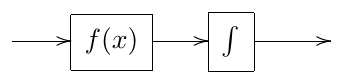
Figure 6.61: Waveshaper immedidately followed by an integrator.
It is interesting to notice that what thereby remains of the integrator is the native integrator contained in Fig. 3.3). Thus, in order to implement an antialiased waveshaper followed by a trapezoidal integrator, simply use a naive integrator instead. This effectively produces trapezoidal integrator, simultaneously “killing” the unwanted latency produced by the antialiased waveshaper.
The solution proposed in Fig. 6.63 works quite well. There is still one subtlety though, which, depending on the circumstances, may be fully academic or not. By “assigning” the functionality of the first part of the integrator to the antialiased waveshaper, we effectively positioned the gain element into the middle of the integrator (Fig. 6.64). This doesn’t affect the time-invariant behavior of the integrator, but will introduce some changes if the cutoff is varying.
In order to avoid that effect, we would need to somehow include the varying into the averaging implemented by (6.38). A straightforward possibility would be to change (6.37) into
(remember that we assume ), where . Trapezoidal integration assumes (kind of) that the signals are varying linearly in between the samples, therefore (6.41) can be rewritten as
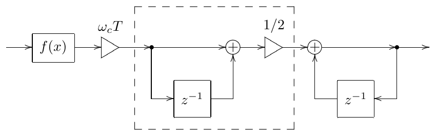
Figure 6.62: Antialiased waveshaper combined with direct form I integrator. The dashed line highlights the part of the integrator which is equivalent to the waveshaper at low signals.
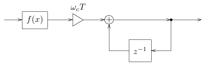
Figure 6.63: Antialiased waveshaper combined with direct form I integrator, the first part of the integrator being dropped, since its implemented by the antialiased waveshaper already.
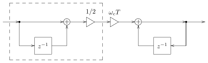
Figure 6.64: Structure in Fig. 6.63 implies positioning the gain element in the middle of the integrator. The dashed line highlights the part which is being replaced by the antialiased waveshaper.
Unfortunately, the formula (6.42) is not fully convincing. At we would expect (6.42) to turn into ordinary trapezoidal integration of yielding
However (6.42) gives in this case
Of course, (6.42) can be further artificially amended. Whether one should attempt anything like that, is an open question.
Waveshaper following an integrator
The opposite order of connection of a waveshaper and an integrator looks much better at first sight, since in this case we could use a transposed direct form I integrator (Fig. 6.65), which won’t require us to reposition the cutoff gain.40
A concern which this approach is raising though, is that, as we have seen, the latency introduced by the waveshaper is caused by the averaging occurring after the nonlinearity, whereas in Fig. 6.65 the averaging in the integrator, which we are dropping, is occurring before the nonlinearity. On the other hand, linear interpolation, which is used to construct from in (6.36), is also having a lowpass filtering effect similar to the one of the averaging, while it doesn’t actually matter, whether we compensate the latency before or after the waveshaper. Therefore Fig. 6.65 may also provide an acceptable solution.
Waveshaper followed by a 1-pole lowpass
Let’s now consider the case of the feedback saturator in Fig. 6.6, where the saturator is not exactly followed by an integrator, but by a complete 1-pole? Fig. 6.66 depicts this situation explicitly showing the internal structure of the 1-pole.
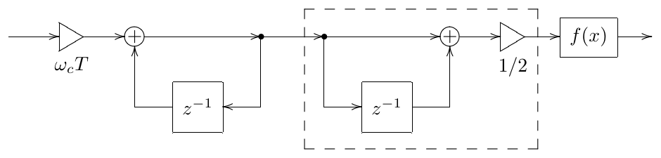
Figure 6.65: Transposed direct form I trapezoidal integrator fol- lowed by a waveshaper. The dashed line highlights the part of the integrator which is about to be dropped.
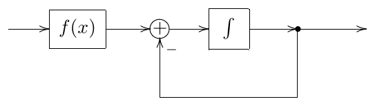
Figure 6.66: Waveshaper followed by a 1-pole lowpass.
Replacing the integrator with its direct form I implementation we obtain the structure in Fig. 6.67. Following the approach of Fig. 6.64, we reposition the element, as shown in Fig. 6.68.
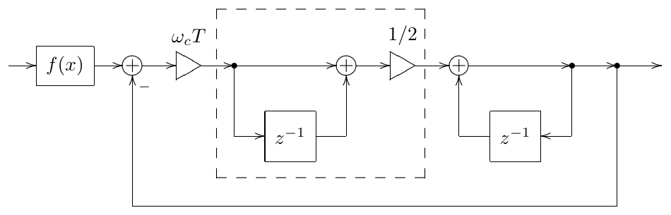
Figure 6.67: Waveshaper followed by a 1-pole lowpass built around a direct form I integrator.
Now we would like to drop the part of the direct form I integrator, but only for the signal coming from the waveshaper. The feedback signal of the 1-pole should still come through the full integrator. This can be achieved by injecting the waveshaped signal into a later point of the feedback loop. The resulting structure in Fig. 6.69 thereby compensates the latency introduced by the antialiased waveshaper.
The structure in Fig. 6.69 can be further simplified as shown in Fig. 6.70, where we “slid” the inverter “-1” all the way through to the injection point of the waveshaped signal. Such change doesn’t cause any noticeable effects.41 Noticing that the two elements in Fig. 6.70 are actually sharing the same input signal, we can combine both into one (Fig. 6.71).
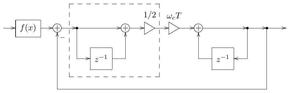
Figure 6.68: Structure from Fig. 6.67 with a changed position of the cutoff gain.
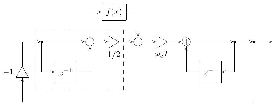
Figure 6.69: Structure from Fig. 6.68 with the waveshaped signal bypassing the first part of the direct form I integrator (thereby compensating the introduced latency).
Fig. 6.71 contains a zero-delay feedback loop, which can be resolved. Let’s introduce helper variables , and as shown in Fig. 6.71 and let . Writing the equations implied by the block diagram we have
from where
Considering that we obtain the structure in Fig. 6.72.
Notice that the obtained structure in Fig. 6.72 is pretty much identical to the structure of the naive 1-pole lowpass filter in Fig. 3.5, except that the cutoff gain is not but . Thus, in order to implement an antialiased waveshaper followed by a 1-pole lowpass, we simply use a naive 1-pole lowpass with adjusted cutoff instead, which effectively “kills” the unwanted latency.
In principle we could have tried to avoid the repositioning of the gain element. Attempting to do so, we could have gone from Fig. 6.67 to the structure in Fig. 6.73. However, this solves only one half of the problem, namely fixing the issue in the feedback path, while the issue is still there for the waveshaped signal. The considerations of possibly including the averaging of into the antialiased waveshaper apply, where we are having exactly the same situation as in the case of an integrator following a waveshaper.
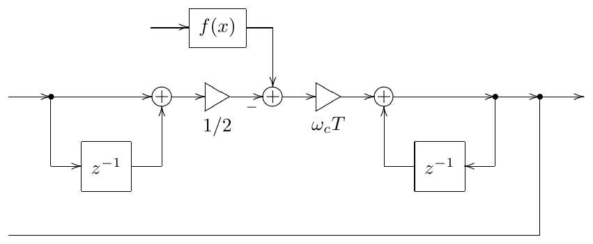
Figure 6.70: Structure from Fig. 6.69 with a changed position of the inverter.
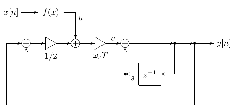
Figure 6.71: Structure from Fig. 6.70 with merged elements.
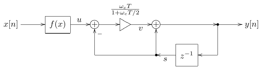
Figure 6.72: Structure from Fig. 6.71 with resolved zero-delay feedback loop, implementing Fig. 6.66 with latency compensation.
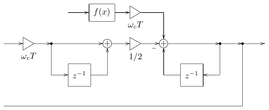
Figure 6.73: Structure from Fig. 6.67 with the waveshaped signal bypassing the first part of the direct form I integrator (thereby compensating the introduced latency) but without repositioning of gain element.
1-pole lowpass followed by a waveshaper
In case of a 1-pole lowpass filter followed by a waveshaper (Fig. 6.74) we can use the transposed direct form I integrator, as we did in Fig. 6.65. The respective structure is shown in Fig. 6.75.
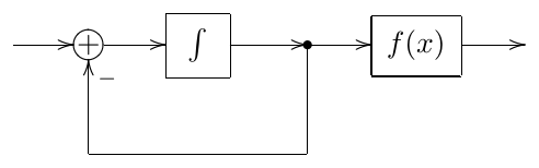
Figure 6.74: 1-pole lowpass followed by a waveshaper.
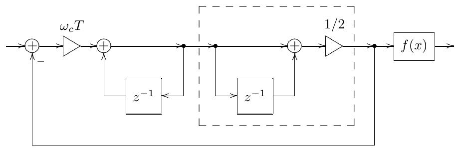
Figure 6.75: 1-pole lowpass built around a transposed direct form I integrator followed by a waveshaper.
In this case we can simply pick up the waveshaper input signal in the middle of the integrator, bypassing the second half (Fig. 6.76). Noticing that the two elements in Fig. 6.76 are picking up the same signal, we could merge them into a single element as shown in Fig. 6.77, thereby producing a direct form II integrator (compare to Fig. 3.9).
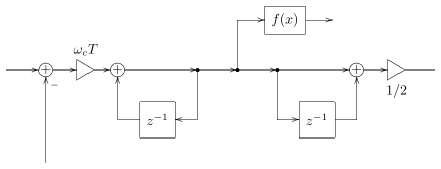
Figure 6.76: Structure from Fig. 6.75 with the waveshaper skipping the second half of the transposed direct form I integrator (thereby compensating the introduced latency).
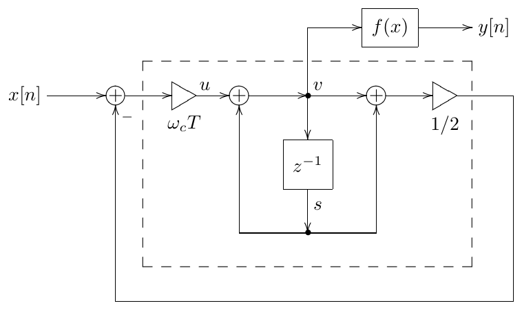
Figure 6.77: Structure from Fig. 6.76 with merged elements. The dashed line highlights the direct form II integrator.
In order to resolve the zero-delay feedback loop in Fig. 6.77 we introduce helper variables , and as shown in Fig. 6.77 and we let . Then, writing the equations implied by the block diagram, we have
from where
Considering that we obtain the structure in Fig. 6.78.
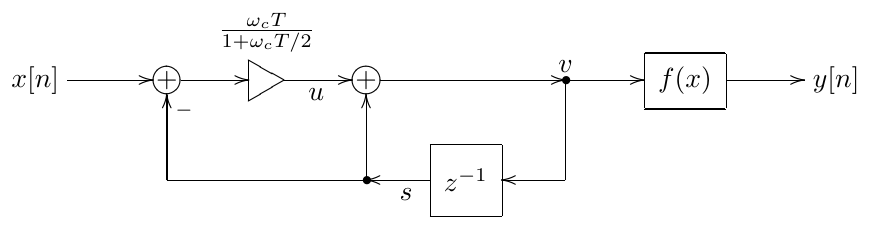
Figure 6.78: Structure from Fig. 6.77 with resolved zero-delay feedback loop, implementing Fig. 6.74 with latency compensation.
Notice that the obtained structure in Fig. 6.78 is identical to the structure in Fig. 6.72, except for the the opposite order of the naive 1-pole lowpass and the waveshaper. Thus, in order to implement a 1-pole lowpass followed by an antialiased waveshaper we simply use a naive 1-pole lowpass with adjusted cutoff instead.
Other positions of waveshaper
In Fig. 6.66 we had a waveshaper followed by a lowpass, but imagine it was a highpass instead (Fig. 6.79).42 In this case, even if we use the tricks similar to the ones we did in the lowpass case, we still won’t be able to eliminate the latency on the feedforward path between and .
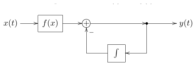
Figure 6.79: Waveshaper followed by a 1-pole highpass.
If there is e.g. a lowpass further after the the highpass:
then we can eliminate the latency by changing the lowpass, exactly as we did before. The highpass filter will work on a signal delayed by half a sample, but this will be compensated in the immediately following lowpass. Similarly, if there is a preceding lowpass:
we could consider compensating the latency by changing that lowpass. The same of course could be done if instead of a lowpass we find an integrator, or a suitable structure containing one.
However it might happen that there is no lowpass or an integrator or any other structure suitable for this purpose, neither after the waveshaper nor before it. In such cases we could artificially insert a 1-pole lowpass immediately before or after the waveshaper (Fig. 6.80), setting the cutoff of this lowpass to a very high value. In this case we could hope that the insertion of the new lowpass would not significantly change the signal, at least not in the audible range, if its cutoff is lying well above.
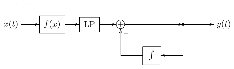
Figure 6.80: Artificially inserted 1-pole lowpass.
One still has to be careful, since such lowpass will introduce noticeable changes into the behavior of the system in the spectral range above the lowpass’s cutoff and even, to an extent, below its cutoff. Even though a lowpass generally reduces the amplitude of signals, due to the changes in the phase it could increase the system’s resonance, causing the system to turn to selfoscillation earlier than expected.43 In a nonlinear system the inaudible parts of the spectrum could become audible through the so-called intermodulation distortion.44 So, it’s a good idea to test for the possible artifacts created by the introduction of such lowpass.
Zero-delay feedback equation
The appearance of antialiased waveshapers in a zero-delay feedback loop creates the question of solving the arising zero-delay feedback equations. Fortunately, this doesn’t create any new problems, as the inistantaneous response of an antialiased waveshaper can be represented in familiear terms.
Indeed, according to (6.38) the instantaneous response of an antialiased waveshaper is simply another waveshaper:
where is the waveshaper function’s parameter, which is having a fixed value at each given time moment . Thus we obtain the already familiar kind of a zero-delay feedback equation with a waveshaper.
Ill-conditioning
If , the denominator of (6.38) will be close to zero. Rather fortunately this also means that the numerator will be close to zero as well, so that, at least formally, their ratio should produce a finite value. However practically this could mean precision losses in the numeric evaluation of the right-hand side of (6.38) (or division by zero if ).
Since , the value of the interpolated signal and respectively the value of shouldn’t change much on and thus the integral in (6.38) can be well approximated by a value of somewhere on that interval.45 In principle we could take any point on that interval, but intuitively we should expect the midway point to give the best result, and thus we take
Notice that at (6.44) turns into (6.39).
The fallback formula (6.44) creates no new problems for the solution of the zero-delay feedback equation, since in instantaneous response terms it looks like another waveshaper
where . Note, however, that when using iterative approaches to the solution of the zero-delay feedback equation, we potentially may need to switch between (6.43) and (6.45) on each iteration step.
The choice between the normal and the ill-conditioned case formulas should depend on the comparison of estimated precision losses in (6.38) and the error in (6.44). In that regard note, that it might be a good idea to choose the antiderivative so that . This could improve the precision of numerical computation of (6.38) and (6.43) at low signal levels, as subtraction of two close numbers is the main source of precision losses here. On the other hand, the main source of error in (6.44) and (6.45) is nonlinear behavior of on the segment lying between and .46
Summary
Nonlinear filters can be constructed by introducing waveshapers into block diagrams. Two important types of waveshapers are saturators and antisaturators. Saturators used in resonating feedback loops prevent the signal level from infinite growth. Antisaturators have a similar effect in damping feedback paths.
The discussed types of usage of saturators in filters included feedback loop saturation, transistor ladder-style 1-pole saturation and OTA-style 1-pole saturation. The discussed usage of antisaturators included the diode clipper-style saturation of 1-poles and the usage in the damping path of an SVF.
Waveshapers usually turn zero-delay feedback equations into transcendental ones, which then need to be solved using approximate or numeric methods, although in some cases analytic solution is possible.
Discrete-time waveshaping produces aliasing, which might need to be mitigated using oversampling and/or some more advanced methods.
-
Sometimes the effect created by discontinuities is explicitly being sought after, e.g. in a rectification waveshaper . ↩
-
Apparently, hard clipper is a compact-range saturator. ↩
-
There doesn’t seem to be a universally accepted definition of which kinds of saturators are referred to as soft clippers, and which aren’t. E.g. the set of soft clippers could be restricted to contain only bounded saturators. In this book we will understand the term soft clipper in the widest possible sense. ↩
-
If the system is in the zero state, then in the absence of the input signal it will stay forever in this state of “unstable equilibrium”. In analog circuits, however, there are always noise signals present in the system, which will excite the transient response components, thus destroying the equilibrium. In the digital implementation such excitations need to be performed manually. This can be done by initializing the system to a not-exactly-zero state, or by sending a short excitation impulse into the system at the initialization, or by mixing some low-level noise at one or multiple points into the system. Often a very small constant DC offset will suffice instead of such noise. ↩
-
As the saturator is effectively reducing the total gain of the feedback loop, at the selfoscillation will first have an infinitely small signal level, where the saturator is transparent. Increasing the value of further we can bring the selfoscillation to an audible level. ↩
-
Notice that, with the saturator positioned in the feedback path, at the filter effectively becomes linear. ↩
-
This observation was made by Dr. Julian Parker. ↩
-
Recall that for a series of 1-pole lowpasses (which denotes in Fig. 6.12) . ↩
-
In a realtime situation it would be a good idea to artificially bound the number of iterations from above. ↩
-
Of course this is not exacty oversampling, because the state of the system (manfesting itself in the variable) is frozen. ↩
-
Clearly, the smoother will not help in the instantaneously unstable case, occurring when . ↩
-
There are a number of tricks which can be employed to improve the convergence of Newton-Raphson, but even those might not help in all situations. The specific tricks can be found in the literature on numerical methods and fall outside the scope of this book. ↩
-
Taking as the unknown to solve for addresses the division by zero issue, but the other issues are similar to the choice of . ↩
-
Treating the error in the numerically computed solution as noise, we can define the signal-to-noise ratio (SNR) as the ratio of the absolute magnitudes of the error and the signal, expressed in decibels. ↩
-
Whether this is too expensive or not depends on a number of factors. E.g. in Newton-Raphson method we needed to compute both and . With the hyperbolic tangent function we were quite fortunate in that the derivative of the function is trivially computable from the function value () and thus doesn’t create significant computation cost. Had the derivative computation been expensive, the computation cost of 10 iterations of bisection could have been comparable to 5 iterations of Newton-Raphson. ↩
-
Proposed for usage in the zero-delay feedback context by Teemu Voipio. ↩
-
This is a particular case of a more general idea, where we would use the result obtained by one of the above approximations as an initial point for an iterative algorithm. ↩
-
We use the implicit form, because the explicit form has some ill-conditioning issues. Besides, in order to solve (6.13) for the specific second-order shaper function , we will need to effectively go from explicit to implicit form during the algebraic transformations of the resulting equation anyway, thus using the explicit form wouldn’t have simplified the solution, but on the contrary, would have made it longer. ↩
-
More precisely, one of the two values. ↩
-
It can be shown, that at which defines the steepness of the asymptote. ↩
-
In the previously discussed case we didn’t have a switch between larger and smaller solutions. But is a limiting case of (6.24) at , so why is there no switch? It turns out that both switches occur simultaneously at (since the oblique asymptote of becomes vertical), and thus we simply always choose the larger solution. ↩
-
Note that the described binary search process doesn’t rely on the regular spacing of breakpoints along the axis. This suggests that we might use an irregular spacing, e.g. placing the breakpoints more densely in the areas of higher curvature. Irregularly spaced breakpoints might complicate the initial bracketing a bit, though. ↩
-
Treating the hard clipper as a piecewise-linear shaper is just a demonstration example. For a hard clipper shape it might be simpler and more practical to simply perform a linearization at zero (thereby treating the hard clipper as a fully transparent shaper ) to find . As the very next step after that is sending through the hard clipper, at the output of the hard clipper we will get the true value, as if we properly solved the equation (6.13) ↩
-
A famous piece of work describing this specific nonlinear model of the transistor ladder filter is the DAFx’04 paper Non-linear digital implementation of the Moog ladder filter by Antti Huovilainen. Therefore this model is sometimes referred to as the “Antti’s model”. ↩
-
It might be a good idea to write the equation system in terms of integrator input signals as an exercise. ↩
-
Going out of supported range of due to numerical errors is more likely to happen in more complicated structures than the one in Fig. 6.54. However since we are using Fig. 6.54 as a demonstration of general principles, we should mention this aspect as well. ↩
-
Of course, we should remember that we already know the output signal of the antisaturator and not attempt to evaluate it again as , which was the whole point of solving for . ↩
-
Note that thereby we can even use an antisaturator which is an inverse of hard clipper. ↩
-
More likely so for a “standalone” saturator being used as an overdrive effect, rather than for a saturator used in a complicated feedback loop structure in a filter. ↩
-
Clearly, by “amplitude” here we don’t mean the momentary value of the signal but rather some kind of average or maximum. ↩
-
Formally the filter would have produced the DC offset of the signal at the output. The fundamental and all other harmonics, being way above filter’s cutoff, would have been filtered out. ↩
-
Or, if we think in terms of real-form Fourier series, where only positive-frequency partials are present, the frequencies of partials of are all possible sums and differences of frequencies of partials of . ↩
-
If the Taylor expansion of has a finite convergence radius, we still can make the same argument about spectrum expansion, at least for the signals which are small enough to fit into the convergence radius of the Taylor series of . Note that we also could expand not around but around some other point , making the same consideration applicable for signals centered around . ↩
-
A discontinuity of -th order derivative generates harmonics rolling off as . Thus a discontinuity in a 2nd derivative generates harmonics at . A discontiuity in the function itself (0th derivative) generates harmonics at (Fourier series of sawtooth and square signals are examples of that). ↩
-
However, it still might reduce the amount of aliasing. ↩
-
Higher sampling rates lead to smaller relative increments of integrator states (at the same cutoff value in Hz). Thus, at some point higher computation precision will be required. 32 bit floats might happen to become insufficient pretty quickly, but 64 bit floats should still do in a wide range of high sampling rates. ↩
-
The approach was proposed independently by A.Huovilainen, E.Le Bivic, Dr. J.Parker and possibly others. The application of the approach within zero-delay feedback context has been developed by the author. ↩
-
Still, 44.1kHz would be usually insufficient and one will need to go to 88.2kHz or even higher. ↩
-
Similarly, linear interpolation can be interpreted in terms of continuous-time lowpass filtering which suppresses the aliasing discrete time spectra. ↩
-
Technically the integrator in Fig. 6.65 is, formally, not exactly a transposed direct form II integrator, as the 1/2 gain element should have been positioned in the middle. However, since this is a constant gain, we can shift it without causing the same concerns as in the case of shifting the potentially varying gain element. ↩
-
The internal state stored in the first element is inverted compared to what it used to be, but this is compensated by the new position of the inverter. ↩
-
The highpass in Fig. 6.79 might look different from the one in Fig. 2.9, however it’s not difficult to realize that in fact both structures are identical. ↩
-
This would be particularly the case in a 4-pole lowpass ladder filter, where the effect is noticeable at ladder filter’s cutoff settings comparable or higher than the cutoff of the added lowpass. ↩
-
Recall that e.g. in (6.33) the output signal of a waveshaper contained all sums and differences of the frequencies of the original signal. Thus if the difference of two frequencies, both lying well above the audible range, falls into the audible range, these originally inaudible partials will create an audible one. ↩
-
This is more precisely stated by the mean value theorem. ↩
-
Note that if is fully linear on that segment, then (6.44) gives the exact answer. One could also obtain an estimation of the error of (6.44) by expanding in Taylor series around and noticing that applying (6.38) just to the first two terms of this expansion gives (6.44) (as the contribution of the first-order term of the series turns out to be zero). Therefore the error of (6.44) is equal to the contribution of the remaining terms of the Taylor series to (6.38). ↩