Chapter 5: Ladder filter
In this chapter we are going to discuss the most classical analog filter model: the transistor ladder filter. The main idea of this structure, which is to create resonance by means of a feedback loop, is encountered in many other filter designs, some of which we are also going to discuss. We will be referring to the class of such filters as simply ladder filters.1
5.1 Analog model
The most classical example of a ladder filter is transistor ladder filter, which implements a 4-pole lowpass structure shown in Fig. 5.1.2 The structure in Fig. 5.1 is not limited to transistor-based analog implementations. Particularly, there are many implementations of the same structure based on OTAs (operational transconductance amplifiers). The difference between transistor- and OTA-based ladders is, however, lying in the nonlinear behavior, which we are not touching at this point yet. The linear aspects of both are identical.
The LP blocks denote four identical (same cutoff) 1-pole lowpass filters (Fig. 2.2). The coefficient controls the amount of negative feedback, which creates resonance in the filter. Typically , although is also sometimes used.

Figure 5.1: Transistor (4-pole lowpass) ladder filter.
Let be the 1-pole lowpass transfer function. Assuming complex exponential and we write from where and the transfer function of the ladder filter is
At the filter behaves as 4 serially connected 1-pole lowpass filters.
The poles of the filter are respectively found from giving where the raising to the 1/4th power is understood in the complex sense, therefore giving 4 different values: (this time is understood in the real sense). Thus there are 4-poles and we can also refer to this filter as a 4-pole lowpass ladder filter.
At all poles are located at , as grows they move apart in 4 straight lines, all going at “ angles” (Fig. 5.2). As grows from 0 to 4 the two of the poles (at ) are moving towards the imaginary axis, producing a resonance peak in the amplitude response (Fig. 5.3). At they hit the imaginary axis: and the filter becomes unstable.3
In Fig. 5.3 one could notice that, as the resonance increases, the filter gain at low frequencies begins to drop. Indeed, substituting into (5.1) we obtain This is a general issue with ladder filter designs.
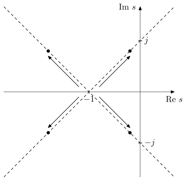
Figure 5.2: Poles of the 4-pole lowpass ladder filter.
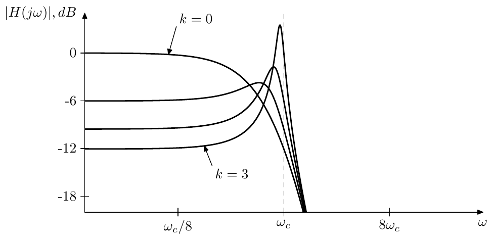
Figure 5.3: Amplitude response of the 4-pole lowpass ladder filter for various .
5.2 Feedback and resonance
Before we continue with discussing more practical aspects of the ladder filter, we’d like to make one important observation considering the resonance peaks created by the ladder filter feedback.
In Fig. 5.3 we can see that, similarly to the 2-pole case, the resonance frequency is approaching the filter cutoff frequency as the filter approaches selfoscillation at . This is a manifestation of a more general principle concerning ladder filters as such. Consider a general ladder filter in Fig. 5.4, where denotes a more or less arbitrary structure, whose transfer function is . Notice that the feedback in Fig. 5.4 is not inverted.
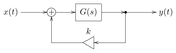
Figure 5.4: Structure of a generic ladder filter.
The transfer function of the entire structure is therefore and the poles are defined by the equation That is at the poles of are the zeros of (the latter obviously simply being the poles of ). As begins to deviate from zero, the solutions of (5.4) will move in the -plane, usually in a continuous fashion. E.g. for the 4-pole lowpass ladder (Fig. 5.1) we had and (5.4) takes the form , where we take instead of because of the inverted feedback in Fig. 5.1.
The value of at which the filter starts to selfoscillate should correspond to some of the poles being located on the imaginary axis. At this moment the infinitely high resonance peak in the amplitude response is occurring exactly at these pole positions. Denoting a purely imaginary pole position as , we rewrite (5.4) for such poles as or We can refer to (5.5) as the selfoscillation equation for a feedback loop. This equation implies that selfoscillation appears at the moment when the total frequency response across the feedback loop exactly equals 1 at some frequency . That is the total amplitude gain must be 1, and the total phase shift must be .
This is actually a pretty remarkable result. Of course it is quite intuitive that selfoscillation tends to occur at frequencies where the feedback signal doesn’t cancel the input signal, but rather boosts it. And such boosting tends to be strongest at frequencies where we have a total phase shift across the feedback loop. However, what is quite counterintuitive, is that selfoscillation can appear (as is reaching the respective threshold value) only at such frequencies.4
Therefore for the selfoscillation appears at frequencies where the phase response of is . For the selfoscillation appears at frequencies where the phase response of is . The respective value of can be found from (5.5) giving or, rewriting (5.6) in terms of the amplitude response of : where we take the plus sign if the phase response of at is and the minus sign if the phase response of at is .
The just discussed effects are the reason that we used negative feedback in the 4-pole lowpass ladder filter. We want the resonance to occur at the filter’s cutoff. The phase response of a single 1-pole lowpass at the cutoff frequency is , respectively the phase response of a chain of four 1-poles is , exactly what we need for the resonance peak, if we use negative feedback.
At the same time, the amplitude response of a 1-pole lowpass at the cutoff is , respectively the amplitude response of a chain of four 1-poles is . According to (5.7), the infinite resonance is attained at .
At a chain of four 1-pole lowpasses will have a phase shift of , while the amplitude response at is 1. Therefore, in Fig. 5.1 the “selfoscillation” at will occur at . However the amplitude response peak at hardly can count as resonance.
5.3 Digital model
A naive digital implementation of the ladder filter shouldn’t pose any problems. We will therefore immediately skip to the TPT approach.
Recalling the instantaneous response of a single 1-pole lowpass filter (3.29), we can construct the instantaneous response of a serial connection of four of such filters. Indeed, let’s denote the instantaneous responses of the respective 1-poles as (obviously, the coefficient is identical for all four, whereas depends on the filter state and therefore cannot be assumed identical). Combining two such filters in series we have Adding the third one: and the fourth one: where Using the obtained instantaneous response of the series of 4 1-poles, we can redraw the ladder filter structure as in Fig. 5.5.
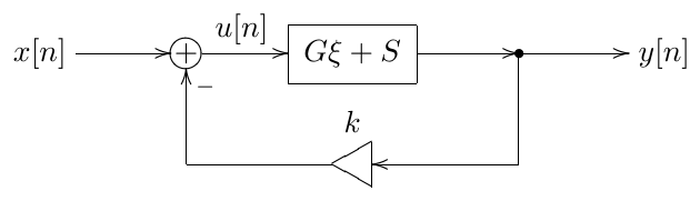
Figure 5.5: TPT 4-pole ladder filter in the instantaneous response form.
Rather than solving for , let’s solve for the signal at the feedback point. From Fig. 5.5 we obtain from where We can then use the obtained value of to process the 1-pole lowpasses one after the other, updating their state, and computing as the output of the fourth lowpass.
Apparently the total instantaneous gain of the zero-delay feedback loop in Fig. 5.5 and in (5.8) is . As we should recall from the discussion of 1-pole lowpass filters, for positive cutoff settings. Respectively and the filter doesn’t become instantaneously unstable provided .
5.4 Feedback shaping
We have observed that at high resonance settings the amplitude gain of the filter at low frequencies drops (Fig. 5.3). An obvious way to fix this problem would be e.g. to boost the input signal by the factor.5 However there’s another way to address the same issue. We could “kill” the feedback for the low frequencies only by introducing a highpass filter into the feedback path (Fig. 5.6). In the simplest case this could be a 1-pole highpass.
The cutoff of the highpass filter can be static or vary along with the cutoff of the lowpasses. The static version has a nice feature that it kills the resonance effect at low frequencies regardless of the master cutoff setting, which may be desirable if the resonance at low frequencies is considered rather unpleasant (Fig. 5.7).

Figure 5.6: Transistor ladder filter with a highpass in the feedback.
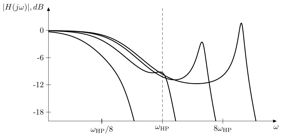
Figure 5.7: Amplitude response of the ladder filter with a static-cutoff highpass in the feedback for various lowpass cutoffs.
In principle one can also use other filter types in the feedback shaping. One has to be careful though, since this changes the total phase and amplitude responses of the feedback path, thus the frequency of the resonance peak and the value of at which selfoscillation is reached may be changed. E.g., quite counterintuitively, inserting a 1-pole lowpass into the feedback path can destabilize an otherwise stable filter.
In order to establish and analyse the latter fact mathematically, we’d need to find the total amplitude response across the feedback loop at the point where the total phase shift is . Let be the underlying 1-pole lowpass of the ladder filter and let be the lowpass in the feedback, with a generally speaking different cutoff . The point is found from the equation where we have used (2.8). The equation (5.9) looks a bit daunting, if having an analytic solution at all. Fortunately, we don’t actually need to know the frequency of the point, it would suffice to know the respective amplitude responses.
Let be the negated phase response of : Expressing as a function of we have . Respectively, expressing the amplitude response as a function of the (negated) phase response we have Thus, the total amplitude response of the four 1-poles in the feedforward path of the ladder filter is and the total phase response of the feedforward path is .
Since (5.10) is cutoff-independent, it also holds for : where , . Now let be the (unknown to us) solution of (5.9), that is the total phase shift at is . In terms of the just introduced functions and equation (5.9) can be rewritten as Since , the phase shift is achieved earlier than without the feedback filter, that is (whatever the value of is).
Computing the total amplitude response of all five 1-pole lowpasses at we have Considering only the first factor we have (where we dropped the argument , understanding it implicitly). Respectively Fig. 5.8 contains the graph of (5.12). The interpretation of this graph is like follows. Suppose the feedback lowpass’s cutoff is very large (). In the limit the feedback lowpass has no effct and As we begin to lower back from the infinity, the value of grows from zero into the positive value range. The graph in Fig. 5.8 plots the total amplitude response of the five 1-pole lowpasses in the feedback loop against the growing . We see that the amplitude response grows for quite a while. As long as it is above 1/4, the filter will explode at . The zero amplitude response at corresponds to , where the extra lowpass is fully closed, thus the entire feedback loop is muted.
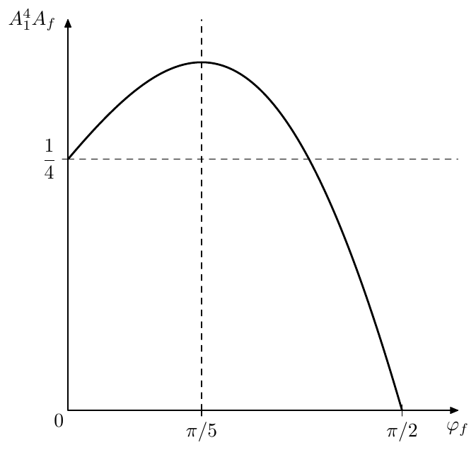
Figure 5.8: Total amplitude response of the four feedforward lowpass 1-poles plus the feedback lowpass 1-pole at the phase shift point, plotted against the phase shift by the feedback 1-pole.
At (equal cutoffs of all 1-poles) from (5.11) we have . In Fig. 5.8 one can see that this is the “most unstable” situation among all possible .
In comparison, if we had a 1-pole highpass in the feedback, then we would have and respectively . Therefore the point would be shifted to the right: . Therefore , while , thus the total amplitude response at the point would decrease and the filter won’t become “more unstable” than it was before the introduction of the extra highpass filter.
5.5 Multimode ladder filter
Warning! The multimode functionality of the ladder filter is a somewhat special feature. There are more straightforward ways to build bandpass and highpass ladders, discussed later in this chapter.
By picking up intermediate signals of the ladder filter as in Fig. 5.9 we obtain the multimode version of this filter.
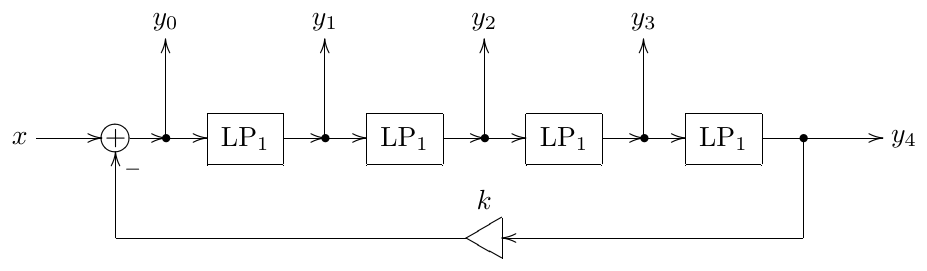
Figure 5.9: Multimode ladder filter.
We then can use linear combinations of signals to produce various kinds of filtered signal.6
Suppose . Apparently, in this case, the respective transfer functions associated with each of the outputs are If then from using the obvious relationship we obtain
4-pole highpass mode
Considering that the 4th order lowpass transfer function (under the assumption ) is built as a product of four 1st order lowpass transfer functions we might decide to build the 4th order highpass transfer function as a product of four 1st order highpass transfer functions : Let’s attempt to build as a linear combination of . Apparently, a linear combination of must have the denominator , so let’s instead construct which at will turn into . We also have while the four zeros at provide a 24dB/oct rolloff at , thus we are still having a more or less reasonable highpass. In order to express as a sum of the modes we write
that is
We need to find from the above equation, which generally can be done by equating the coefficients at equal powers of in the left- and right-hand sides. However, for the specific equation that we’re having here we could do a shortcut by simply formally replacing by (and respectively by ):
from where immediately
The amplitude response corresponding to (5.15) is plotted in Fig. 5.10.
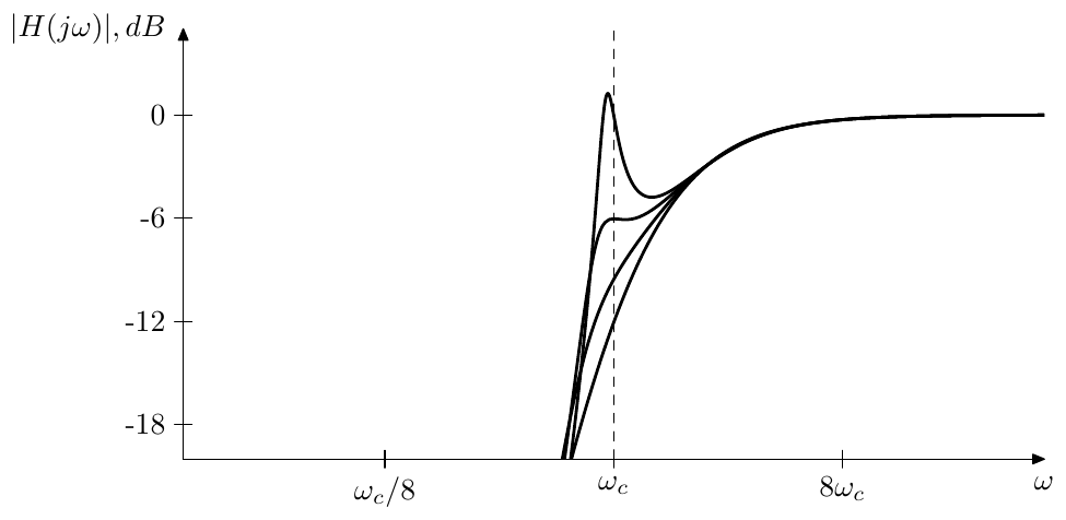
Figure 5.10: Amplitude response of the highpass mode of the ladder filter for various k.
4-pole bandpass mode
A bandpass filter can be built as
The two zeros at will provide for a dB/oct rolloff at low frequencies and will reduce the dB/oct rolloff at high frequencies to the same dB/oct. Notice that the phase response at the cutoff is zero:
The coefficients are found from
The amplitude response corresponding to (5.16) is plotted in Fig. 5.11.
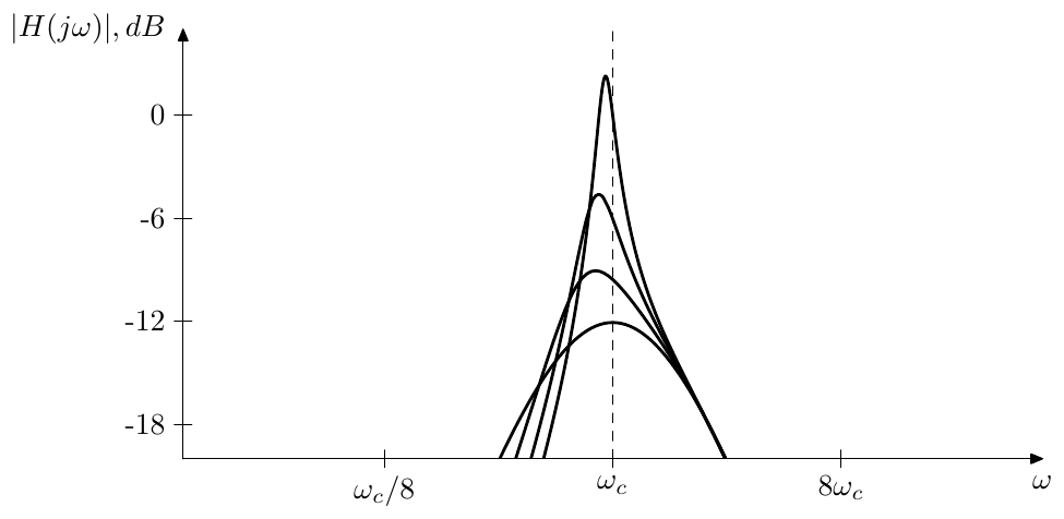
Figure 5.11: Amplitude response of the bandpass mode of the ladder filter for various k.
Lower-order modes
Recalling the transfer functions of the modal outputs in the absence of the resonance (5.13), we can consider the modal signals and their respective transfer functions (5.14) as a kind of “-pole lowpass filters with 4-pole resonance”.
“Lower-order” highpasses can be build by considering the zero-resonance transfer functions
which for turn into
In a similar way we can build a “2-pole” bandpass
Other modes
Continuing in the same fashion we can build further modes (the transfer functions are given for ):
| Transfer function | Mode |
|---|---|
| 3-pole bandpass, 6/12 dB/oct | |
| 3-pole bandpass, 12/6 dB/oct | |
| band-shelving | |
| notch | |
| notch | |
| 2 notches, neutral setting | |
| 2-pole lowpass + notch | |
| 2-pole highpass + notch | |
| 2-pole bandpass + notch |
etc. The principles are more or less similar. We are trying to attain a desired asymptotic behavior at and by having the necessary orders and coefficients of the lowest-order and highest-order terms in the numerator. E.g. by having as the lowest-order term of the numerator we ensure a 12dB/oct rolloff at , or by having as the highest-order term we ensure . The notch at is generated by placing a zero at . The 2-notch version is obtained by explicitly writing out the transfer function of a 4-pole multinotch described in Section 11.3.
5.6 HP ladder
Performing an LP to HP transformation on the lowpass ladder filter we effectively perform it on each of the underlying 1-pole lowpasses, thus turning them into 1-pole highpasses. Thereby we obtain a “true” highpass ladder filter (Fig. 5.12). Obviously, the amplitude response of the ladder highpass is symmetric to the amplitude response of the ladder lowpass (Fig. 5.13).

Figure 5.12: A “true” highpass ladder filter.
The instantaneous gain of a 1-pole highpass is complementary to the instantaneous gain of the 1-pole lowpass:
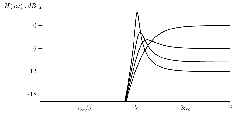
Figure 5.13: Amplitude response of the 4-pole highpass ladder filter for various k.
where . Thus the instantaneous gain of a single 1-pole highpass is varying within the range and so does the gain of the chain of four highpasses: . Therefore, 4-pole highpass ladder doesn’t get instantaneously unstable for .
5.7 BP ladder
In order to build a “true” 4-pole bandpass ladder, we replace only half of the lowpasses with highpasses (it doesn’t matter which two of the four 1-pole lowpasses are replaced). The total transfer function of the feedforward path is thereby
where each of the factors is built from a serial combination of a 1-pole lowpass and a 1-pole highpass:
Apparently is a 2-pole bandpass with damping and a serial combination of two of them makes a 4-pole bandpass. The frequency response of at is , that is there is no phase-shift. Respectively the frequency response of at is , also without a phase shift. Therefore we need to use positive rather than negative feedback (Fig. 5.14), the selfoscillation still occuring at , the same as with lowpass and highpass ladders.

Figure 5.14: A “true” bandpass ladder filter.
Noticing that the filter structure is invariant relative to the LP to HP transformation, we conclude that its amplitude response must be symmetric (around ) in the logarithmic frequency scale (Fig. 5.15).
The question of instantaneous instability is more critical for the bandpass ladder, since the feedback is positive. The instantaneous gain of a lowpass-highpass pair is a product of the instantaneous gains of a 1-pole lowpass and a
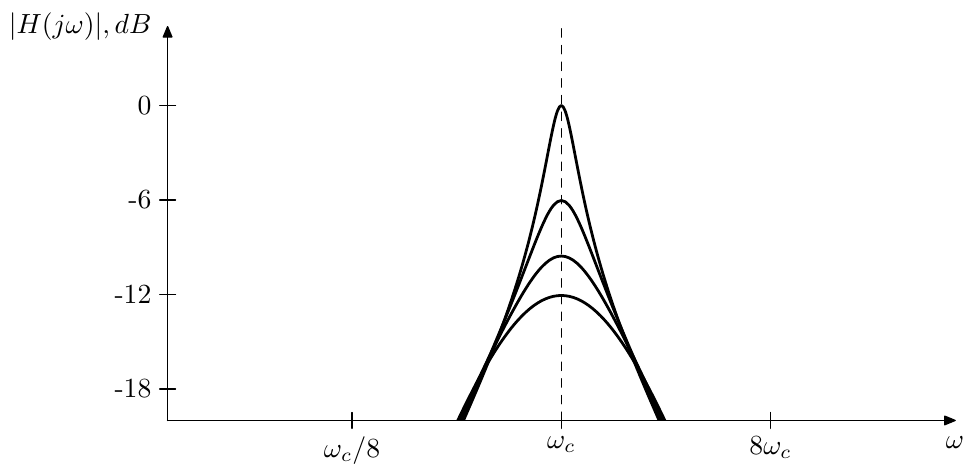
Figure 5.15: Amplitude response of the 4-pole bandpass ladder filter for various k.
1-pole highpass:
(where ). It’s not difficult to verify that the maximum gain of this pair is attained at and is equal to . The maximum instantaneous gain of two of these pairs is therefore , and thus the instantaneously unstable case doesn’t occur provided .
Bandwidth control
Using (5.3) and the fact that the frequency response of at is we obtain the frequency response of the 4-pole bandpass ladder at the cutoff
Therefore, by multiplying the output (or the input signal) of the 4-pole bandpass ladder by we can turn it into a normalized bandpass, where the bandwidth is controlled by varying .
There is another way, however. Recall that the normalized 2-pole bandpass (4.15) is an LP to BP transformation of the 1-pole lowpass . At the same time,
is simply a halved version of (4.15) taken at and therefore is an LP to BP transformation fo the halved 1-pole lowpass . This means that Fig. 5.14 can be replaced by Fig. 5.16 which in turn is an LP to BP transformation of Fig. 5.17.
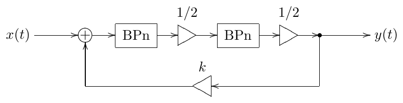
Figure 5.16: 4-pole bandpass ladder filter expressed in terms of normalized 2-pole bandpasses.
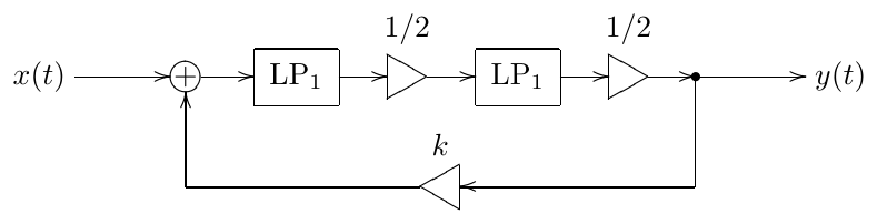
Figure 5.17: LP to BP transformation applied to this structure produces the 4-pole bandpass ladder in Fig. 5.16.
We don’t even specifically care to analyse the structure Fig. 5.17. What is important is that the damping parameter of the LP to BP transformation controls the transformation bandwidth and thereby the bandwidth of the bandpass ladder in Fig. 5.16. Thus, introducing the damping control into the normalized 2-pole bandpasses in Fig. 5.16 we can control the bandpass ladder’s bandwidth by simply varying the damping parameter of the underlying 2-pole bandpasses.
At the same time we still have the parameter available, which we still can use to control the bandwidth of the normalized bandpass (Fig. 5.18). Thus, and provide two different ways of bandwidth control, resulting in somewhat different amplitude response shapes (Fig. 5.19).7
Obviously, normalized 2-pole bandpasses with damping control could be implemented using an SVF. If nonlinearities are involved, however, using TSK/SKF 2-pole bandpasses might be a better option. Since we didn’t introduce the latter yet, we need to postpone the respective discussion. We will return to this question, however, in the discussion of 8-pole bandpass ladder in Section 5.9, where the bandwidth control via the 2-pole bandpass damping will be a particularly desired feature compared to being somewhat academic in the case of a 4-pole bandpass.
5.8 Sallen-Key filters
In this section we are going to introduce two special kinds of 2-pole bandpass ladder filters, the Sallen-Key filter and its transpose.8 They are important because of their nonlinear versions, since, as linear digital 2-pole filters go, the SVF filter could be sufficient for most applications, and it also provides probably the best performance among different TPT 2-poles.
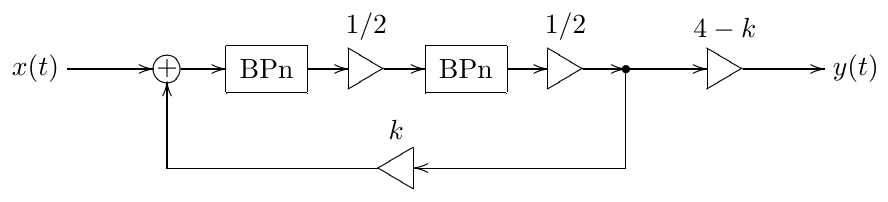
Figure 5.18: 4-pole normalized bandpass ladder filter expressed in terms of normalized 2-pole bandpasses.
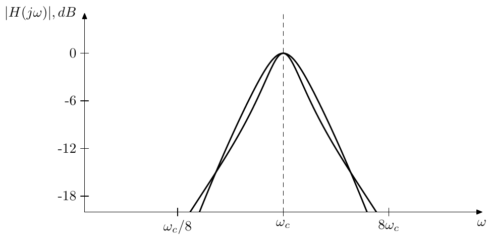
Figure 5.19: Amplitude response of the 4-pole normalized bandpass ladder filter in Fig. 5.18 for two different combinations of and resulting in comparable bandwidths.
For now we shall develop the linear versions of these filters. The Sallen-Key filter is more famous than its transpose, but we’ll start with the transpose, for the sake of a more systematic presentation of the material.
Transposed Sallen-Key (TSK) filters
Attempting to build a 2-pole lowpass ladder filter (Fig. 5.20) we don’t end up with a useful filter.
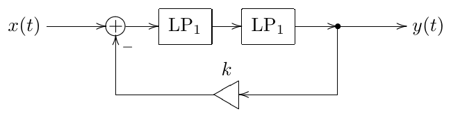
Figure 5.20: 2-pole lowpass ladder filter (not very useful).
Indeed, the transfer function of this filter is
and the poles are respectively at
Interpreting these pole positions in terms of 2-pole cutoff and damping (which we can do using (4.13)), we obtain
Thus, firstly, there is coupling between the feedback amount and the effective cutoff of the filter. Secondly, as grows, stays strictly positive, thus the filter poles never go into the right semiplane (and, as with the 4-pole ladder filter, this would be quite desired once we make the filter nonlinear). So, all in all, not a very useful structure.
A similar situation occurs in an attempt to use two 1-pole highpasses instead of two 1-pole lowpass in the same structure (the readers may wish verify this on their own as an exercise).
This result is no wonder, considering that the transfer function of a chain of two 1-pole lowpasses is , with the phase response being only at and being only at (for the highpasses the situation is opposite, we have only at and only at , which doesn’t make a big difference for our purposes). Thus we don’t get a good resonance peak at any finite location. This however hints at the idea that we might still try to build a 2-pole bandpass ladder filter from a chain of a 1-pole lowpass and a 1-pole highpass, as the total phase shift at the cutoff would be in this case:
The respective structure is shown in Fig. 5.21. Notice that we don’t invert the feedback.
Computing the transfer function of this filter we have
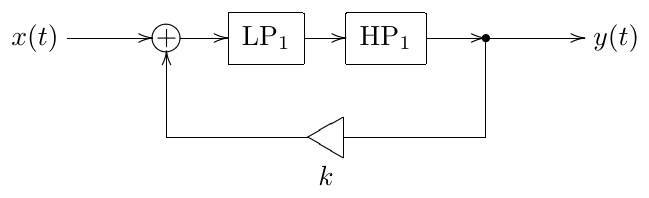
Figure 5.21: 2-pole bandpass ladder filter.
The obtained expression is identical to the transfer function of a 2-pole bandpass filter with a damping gain . That is, the filter in Fig. 5.21 is pretty much the same as a linear 2-pole SVF bandpass, at least from the frequency response perspective. Notice that corresponds to the resonance-neutral setting () while is the self-oscillation point (). As we should remember from the 4-pole bandpass ladder discussion, the maximum possible instantaneous gain of the lowpass-highpass pair is , therefore under the condition the TPT implementation of Fig. 5.21 doesn’t become instantaneously unstable.
It might seem that we have failed to construct a 2-pole lowpass filter using the above approach, but in fact with a slight modification we can obtain one from the bandpass filter in Fig. 5.21. Let’s replace the 1-pole highpass with a 1-pole multimode with highpass and lowpass outputs (Fig. 5.22).
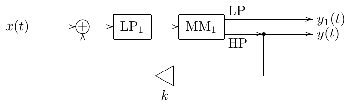
Figure 5.22: 2-pole bandpass ladder filter with an extra output mode.
Obviously, the signal is not affected by this replacement. Let’s find out what kind of signal is . In order to simplify the computation of the transfer function of the entire structure at , consider first the transfer functions of the 1-pole multimode filter used in isolation:
or, for complex sinusoidal signals of the form
where is the input signal of the multimode 1-pole and and are the respective output signals. This means that
Therefore a similar relationship exists between the outputs and of the filter in Fig. 5.22:
and there is the same relationship between their respective transfer functions
where the the transfer function for the signal in respect to the input signal . Therefore is an ordinary 2-pole lowpass signal with damping gain .
Thus we have obtained a multimode 2-pole ladder filter with the lowpass and bandpass outputs. We redraw the structure in Fig. 5.22 once again as Fig. 5.23 to reflect what we have just found out about this structure.
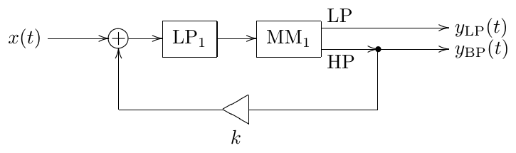
Figure 5.23: Transposed Sallen-Key (TSK) filter.
The structure in Fig. 5.23 happens to be a transpose of the Sallen-Key filter, therefore we will refer to it as the transposed Sallen-Key (TSK) filter.9 The transfer functions of the TSK filter are, as we have found out:
A 2-pole highpass output mode cannot be picked up in a straightforward way, but can be obtained with some extra effort. Let’s also turn the first lowpass into a multimode (Fig. 5.24). It is not difficult to realize that the transfer function for the signal at the LP output of , which is simultaneously the input signal of , is
respectively for the signal at the HP output of we have
Thus we obtain
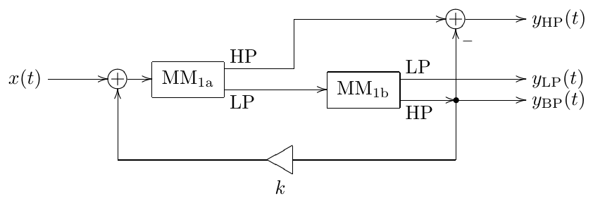
Figure 5.24: Fully multimode TSK filter.
Alternative representations
Recall that 1-pole highpass signal can be obtained as the difference of the 1-pole lowpass filter’s input and output signals:
Then we can replace the multimode 1-pole in Fig. 5.23 by a 1-pole lowpass, constructing the highpass signal “manually” by subtracting the lowpass output from the lowpass input (Fig. 5.25). A further modification of Fig. 5.25 is formally using negative feedback (Fig. 5.26)
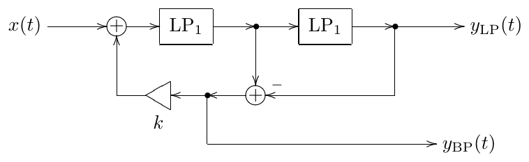
Figure 5.25: TSK filter (alternative representation).
Highpass TSK filter
Let’s take the filter in Fig. 5.21 and switch the order of lowpass and highpass 1-pole filters (Fig. 5.27). Since this doesn’t change the transfer function of the entire chain of 1-poles, the filter output stays the same, it is still a 2-pole bandpass.
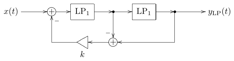
Figure 5.26: TSK filter (alternative representation, negative feedback form).
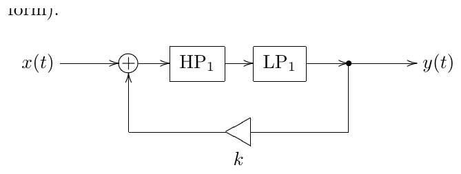
Figure 5.27: 2-pole bandpass ladder filter with a different order of 1-pole lowpass and highpass filters.
Turning the 1-pole lowpass into a multimode we obtain the structure in Fig. 5.28. It’s not difficult to see that the signal at the other output of the multimode is a 2-pole highpass one. Therefore, in order to distinguish between the filters in Figs. 5.23 and 5.28 we will refer to the former more specifically as a lowpass TSK filter and to the latter as a highpass TSK filter. If necessary, we can add the lowpass output, using a way similar to Fig. 5.24.
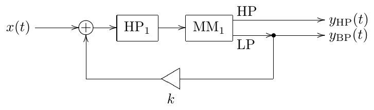
Figure 5.28: Highpass TSK filter.
The highpass versions of Fig. 5.25 and Fig. 5.26 could have been built by performing transformations of Fig. 5.28 similarly to how we did with Fig. 5.23. However it’s easier just to apply the LP to HP substitution () to Figs. 5.25 and 5.26.
Sallen-Key filter (SKF)
We could take the structure in Fig. 5.27 and convert the 1-pole highpass filter into a tranposed multimode 1-pole (Fig. 5.29). By doing this one obtains a transpose of Fig. 5.23 which is (apparently) called Sallen-Key filter or shortly SKF. If necessary, the highpass input can be added, turning Fig. 5.23 into a transpose of Fig. 5.24.
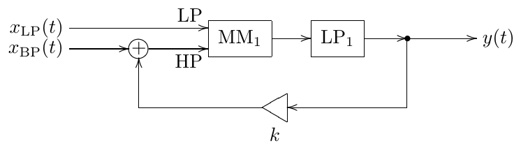
Figure 5.29: Sallen-Key filter.
If instead we take the structure in Fig. 5.21 and convert the lowpass into a transposed multimode 1-pole, we can obtain the structure in Fig. 5.30. In order to distinguish between Fig. 5.29 and Fig. 5.30, we will, as we did with their transposes, refer to the structure in Fig. 5.29 more specifically as a lowpass Sallen-Key filter and to the structure in Fig. 5.30 as a highpass Sallen-Key filter. The lowpass input can be added to the highpass SKF using the transposed version of the idea of Fig. 5.24.
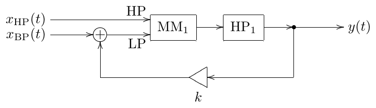
Figure 5.30: Highpass SKF.
The transposed versions of Fig. 5.25 and Fig. 5.26 make alternative representations of the lowpass SKF. E.g. by transposing the structure in Fig. 5.25 we obtain the one in Fig. 5.31.
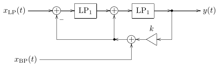
Figure 5.31: Sallen-Key filter (alternative representation).
MIMO Sallen-Key filters
By turning both 1-poles in Fig. 5.27 into multimodes we’ll obtain a MIMO (multiple input multiple output) Sallen-Key filter, as illustrated in Fig. 5.32.
Note that the labelling of the inputs and outputs , , , is thereby formal. The actual transfer functions are defined for signal paths from a given input to a given output:
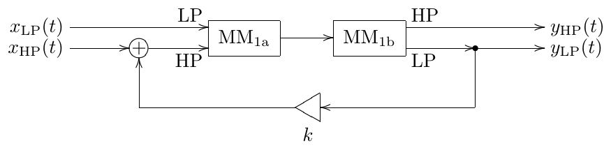
Figure 5.32: MIMO Sallen-Key filter (HP-LP).
| 2-pole lowpass | 2-pole bandpass | |
| 2-pole bandpass | 2-pole highpass |
By putting the feedback path around lowpass-highpass chain rather than lowpass-highpass, Fig. 5.32 is turned into Fig. 5.33.
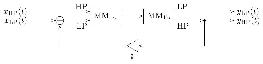
Figure 5.33: MIMO Sallen-Key filter (LP-HP).
Allpass TSK/SKF
Consider again the 2-pole bandpass ladder filter structure in Fig. 5.21. Suppose that we use 1-pole allpasses instead of low- and highpass filters. We also use negative, rather than positive feedback, although this is more a matter of convention. The result is shown in Fig. 5.34, where we also prepared the modal outputs.
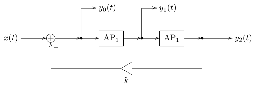
Figure 5.34: 2-pole ladder filter based on allpasses (not so useful).
The transfer function of the main output is
which is not exactly a 2-pole allpass transfer function. The denominator of however looks pretty usable, it’s a classical 2-pole transfer function denominator with damping .
The transfer functions at the other two outputs can be obtained by “reverse application” of the transfer functions of the 1-pole allpasses to :
We can try building the desired transfer function
as a linear combination of , and :
Noticing that the denominators of , , are all identical to the desired denominator already, we can discard the common denominator from the equation and simply write:
or
From where , , . Thus
and the corresponding structure is shown in Fig. 5.35.10 11 The main idea of this structure is very similar to the one of a TSK filter with some “embedded” modal mixture. For that reason we can refer to the filter Fig. 5.35 as a allpass TSK filter, or we could call it a 2-pole allpass ladder filter.
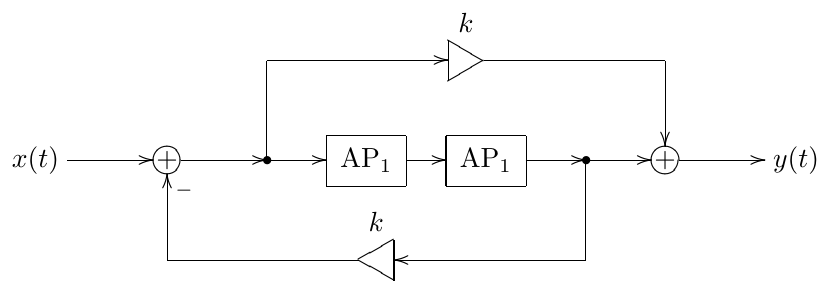
Figure 5.35: Allpass TSK filter.
The 2-pole damping parameter is related to via
so that for the damping varies from to . The stable range corresponds to .
Transposing the structure in Fig. 5.35 we obtain the structure Fig. 5.36 which for obvious reasons we will refer to as an allpass SKF.
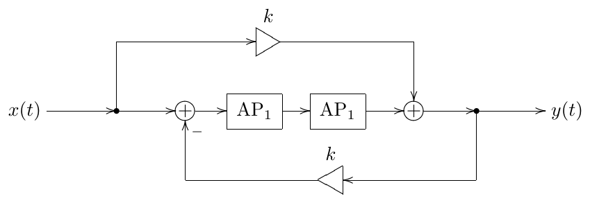
Figure 5.36: Allpass SKF.
5.9 8-pole ladder
Connecting eight 1-pole lowpass filters in series instead of four we can build an 8-pole lowpass ladder filter (Fig. 5.37).
The transfer function of the 8-pole lowpass ladder is obviously
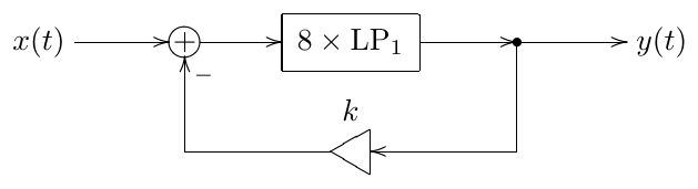
Figure 5.37: 8-pole lowpass ladder filter.
and the pole positions are defined by
giving
where is understood in the multivalued complex root sense:
where
The main difference from the 4-pole ladder lowpass, besides the steeper cutoff slope, is that the phase shift by the chain of 1-pole lowpasses is no longer occurring at the cutoff. Instead, the phase response of the lowpass chain at the cutoff is . In order to find the frequency at which phase shift is occurring we need to solve
that is
(apparently the values an larger cannot be attained by ). This gives
The value of can be easily found using the formula for the tangent of double angle:
where letting we obtain
For we can use the formula for the tangent of the complementary angle:
Thus the resonance peak can occur at . Let’s find the values of at which the respective poles hit the imaginary axis. According to (5.7), is the reciprocal of the amplitude amplitude response of the chain of eight 1-pole lowpasses at the respective frequencies:
finally giving
Thus the selfoscillation at is occurring way much earlier than the one at . It is very unlikely that even in a nonlinear version of this filter, which allows going into unstable range of , we will use as large as 2174. It also hints to the fact that the second resonance is way much weaker than the first one. Therefore, for practical purposes we will simply ignore the second resonance and say that the infinite resonance is occuring at at . Fig. 5.38 illustrates the amplitude response behavior for various .
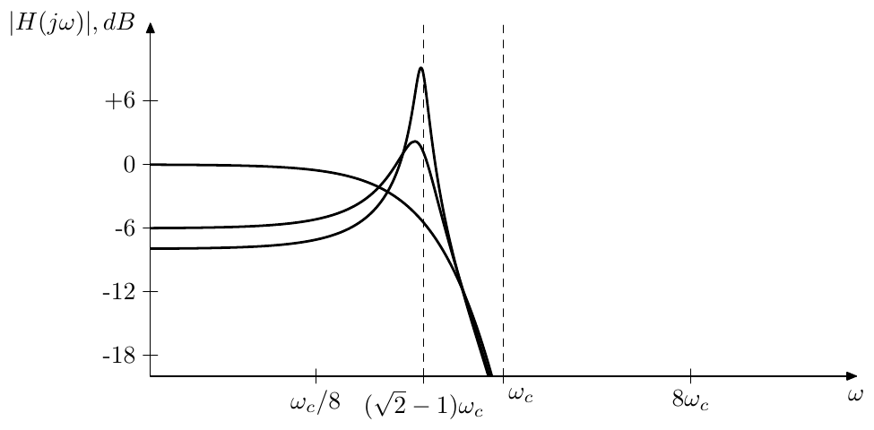
Figure 5.38: Amplitude response of the 8-pole lowpass ladder filter for various .
Considering that at the amplitude response of a chain of eight 1-poles at the cutoff is , which is ca. dB, we could treat the resonance frequency as the “user-facing” cutoff frequency instead, and in practical implementations of the filter let the cutoff of the underlying 1-poles equal the “user-facing” cutoff multiplied by .
One could ask the following question: the phase response of the chain of eight 1-poles at is , therefore why don’t we simply use positive feedback to create the resonance peak at ? The problem is that the phase response at is also . Since the amplitude response at is 1, the selfoscillation will occur already at , whereas at it will occur only at .
The instantaneously unstable range of is found similarly to the 4-pole lowpass ladder and is .
Various modal mixtures for the 8-pole lowpass ladder filter can be built in a similar way to the 4-pole ladder filter. However the fact that the resonance frequency is noticeably lower than the cutoff frequency of the underlying 1-poles will affect the shapes of the resulting modal mixtures. Some smart playing around with the modal mixture coefficients can sometimes reduce the effect of this discrepancy.
8-pole highpass ladder
Replacing the 1-pole lowpasses with highpasses we obtain an 8-pole highpass ladder filter (Fig. 5.39). As we already know from the discussion of the 4-pole highpass, it essentially the same as lowpass except for the substitution. The instantaneously unstable range of is found similarly to the 4-pole highpass ladder and is .
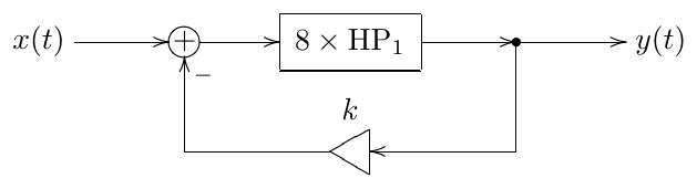
Figure 5.39: 8-pole highpass ladder filter.
8-pole bandpass ladder
Replacing half of the lowpasses with highpasses in Fig. 5.37 we obtain the 8-pole bandpass ladder filter, where we shouldn’t forget that in a bandpass ladder the feedback shouldn’t be inverted (Fig. 5.40).
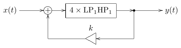
Figure 5.40: 8-pole bandpass ladder filter.
The total gain at the cutoff of the 1-pole chain is
therefore selfoscillation occurs at . Fig. 5.41 illustrates the amplitude response behavior at various . Note that the amplitude response is pretty low (particularly, for it peaks at dB), therefore additional boosting of the output signal may be necessary in practical usage.
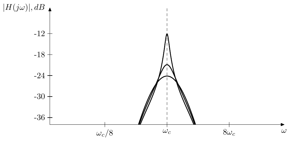
Figure 5.41: Amplitude response of the 8-pole bandpass ladder filter for various .
The instantaneously unstable range of is found similarly to the 4-pole bandpass ladder and is .
An interesting feature of the 8-pole bandpass ladder is that at negative the filter obtains two resonance peaks (Fig. 5.42).12 Indeed, notice that the phase response of the 8-pole lowpass-highpass chain is the same as the one of the 8-pole lowpass chain:
Thus we still have a phase shift at .
The amplitude response of a single lowpass-highpass pair at is
therefore selfoscillation occurs at .
8-pole bandpass ladder with bandwidth control
The occurence of two resonance peaks in an 8-pole bandpass ladder at motivates the introduction of the possibility to control the distance between these two peaks. In Section 5.7 we have introduced two different approaches to control the 4-pole bandpass ladder’s bandwidth. Apparently, the approach using the parameter is not good for our goal here, since we don’t want to affect the amplitude response shape in the vertical direction. Also, from Fig. 5.42 it seems that the variation of k in the negative range has little effect on the actual bandwidth. On the other hand, the approach using the damping of the underlying 2-pole bandpasses looks much more promising.
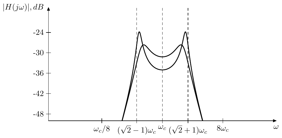
Figure 5.42: Amplitude response of the 8-pole bandpass ladder filter for various k < 0.
Representing the 8-pole bandpass ladder in terms of normalized 2-pole bandpasses (Fig. 5.43) we notice that it is an LP to BP transformation of the filter in Fig. 5.44. The filter in Fig. 5.44 is essentially the same as the ordinary 4-pole lowpass ladder (Fig. 5.1), except that
- the feedback is positive, so that selfoscillation at occurs at some negative value of
- the output signal amplitude and the feedback amount are 16 times lower, thus selfoscillation at doesn’t occur at but at (which matches the already established fact of selfoscillation of Fig. 5.40 and equivalently Fig. 5.43 at ).
Therefore by controlling the bandwidth of the LP to BP transformation, we will control the distance between the resonance peaks in Fig. 5.42.
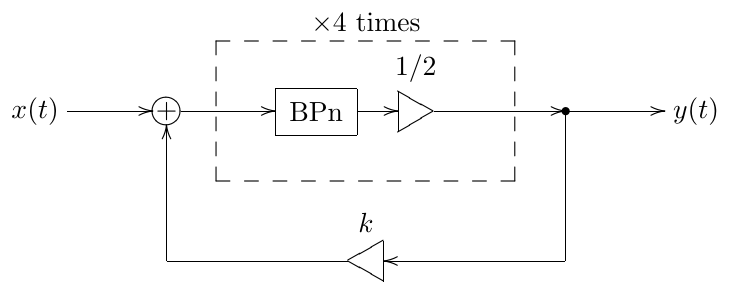
Figure 5.43: 8-pole bandpass ladder filter expressed in terms of normalized 2-pole bandpasses.
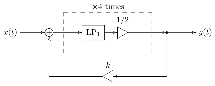
Figure 5.44: 4-pole lowpass ladder filter with positive feedback and additional gains of 1/2. The LP to BP substitution applied to this filter produces the filter in Fig. 5.43.
Since the resonance peak in Fig. 5.44 is occurring at , the formula (4.20) expresses in terms of the distance between the two images of this peak after the LP to BP transformation. Therefore we can directly use the formula (4.20) to control the distance between the resonance peaks in Fig. 5.43. The prewarping techniques described in Section 4.6 also apply, thereby allowing us to achieve the exact positioning of the resonance peaks (in the limit ).
There is an important question concerning the choice of the specific topology for the normalized bandpasses BPn. Of course, the most obvious choice would be to use an SVF. This should work completely fine in the linear case. In a nonlinear case, however, we might want to use a different topology. Particularly, we might want that at our controlled-bandwidth topology becomes fully identical to Fig. 5.40 (therefore obtaining the sound, which is identical to the one of the structure in Fig. 5.40 even in the presence of nonlinear effects).
Assuming that Fig. 5.40 implies interleaved 1-pole low- and highpasses (as shown in Fig. 5.45), a good solution is provided by the TSK/SKF filters. E.g. considering the structure in Fig. 5.21 (which is essentially the TSK filter from Fig. 5.23), we can notice that at it becomes fully equivalent to a single lowpass-highpass pair. This suggests that we could use this structure to construct a halved normalized bandpass (Fig. 5.46), where expressing the TSK feedback in terms of damping we have . Note that at not only the feedback path in Fig. 5.46 is disabled, but also the output gain element is becoming transparent. Using the halved normalized bandpass in Fig. 5.46, we could reimplement Fig. 5.45 as Fig. 5.47.
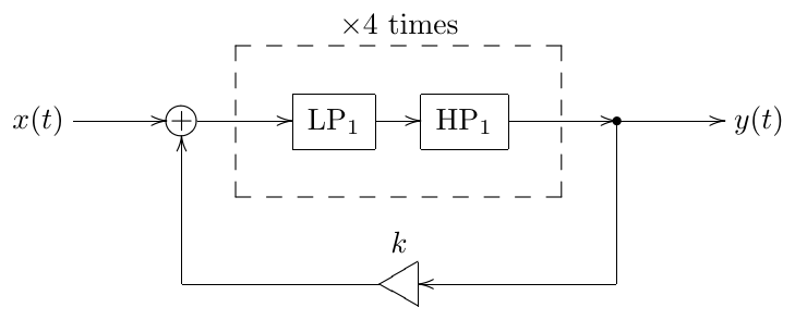
Figure 5.45: Fig. 5.40 implemented by interleaved 1-pole low- and high-passes.
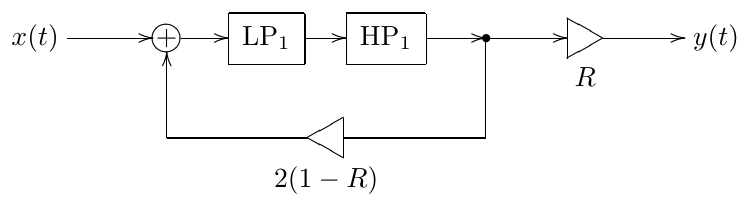
Figure 5.46: Halved normalized TSK bandpass.
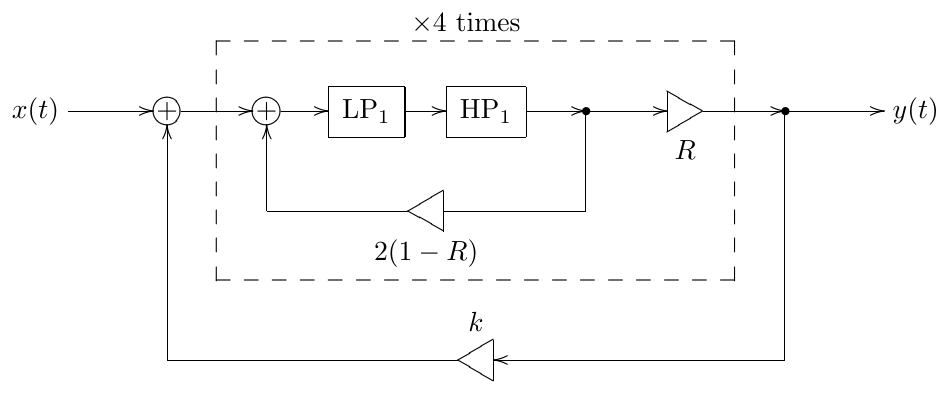
Figure 5.47: 8-pole bandpass ladder filter expressed in terms of halved normalized TSK bandpasses.
5.10 Diode ladder
In the diode ladder filter the serial connection of four 1-pole lowpass filters (implemented by the transistor ladder) is replaced by a more complicated structure of 1-pole filters (implemented by the diode ladder). The block diagram of the diode ladder is shown in Fig. 5.48, while the diode ladder filter adds the feedback loop around that structure, feeding the fourth output of the diode ladder into the diode ladder’s input (Fig. 5.49).
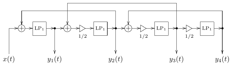
Figure 5.48: Diode ladder.
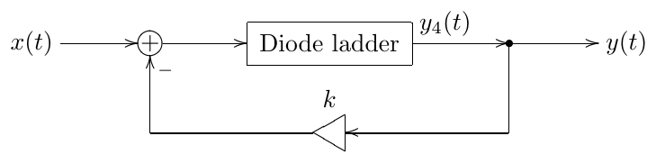
Figure 5.49: Diode ladder filter.
It is instructive to write out the 1-pole equations implied by Fig. 5.48:
In this form it’s easier to guess the reason for the gain elements 1/2 used in Fig. 5.48, they perform the averaging between the feedforward and feedback signals. However this averaging in (5.18) and Fig. 5.48 is not done fully consistently. It would have been more consistent to have no 1/2 gain element at the input of the fourth lowpass, rather than of the first one:
in which case the first lowpass would take as its input, the second lowpass would take as its input, the third lowpass would take as its input, and the fourth lowpass would take as its input. However, (5.18) is a more traditional way to implement a diode ladder filter. Anyway, the difference between (5.18) and (5.19) is actually not that large, since (as we are going to show below) they result in one and the same transfer function,
The more complicated connections between the 1-pole lowpasses present in the diode ladder “destroy” the frequency response of the ladder in a remarkable form, which, is responsible for the characteristic diode ladder filter sound.13 Generally, the behavior of the diode ladder filter is less “straightforward” than the one of the transistor ladder filter.
Transfer function
We are going to develop the transfer function for the diode ladder in a generalized form (Fig. 5.50), where denote blocks with respective transfer functions. In the case of Fig. 5.48 and (5.18) we would have
while in the case of (5.19) we would respectively have
where
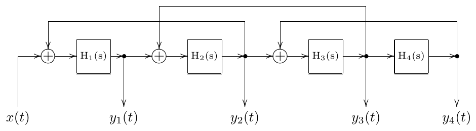
Figure 5.50: Generalized diode ladder in transfer function form.
Assuming complex exponential signals , for the block we have
(where is short for ), therefore
For the block we have
Substituting (5.23) we have
where is a short notation for .
For the block we have
Substituting (5.23) and (5.24) we have
For the block we have
Substituting (5.24) and (5.25) we have
where is the diode ladder’s transfer function. It is easy to see that substituting (5.20) or (5.21) into (5.26) gives identical results, therefore transfer functions arising out of (5.18) and (5.19) are identical. Formula (5.26) also gives one more hint at the reason to use a 1/2 gain with all 1-poles except the first or the last one, as in this case we get unit amplitude response at :
Since we are specifically interested in Fig. 5.48, let’s write its transfer function in a more detailed form. Substituting first (5.20) and then (5.22) into (5.26) we have
where is the fourth-order Chebyshev polynomial.14 The poles of are therefore found from or where are the roots of the Chebyshev polynomial :
Therefore the poles of are purely real and located within :
Since the poles of are located on the negative real semiaxis and there are no zeros, is monotonically decreasing to zero on . Thus is a lowpass.15
In Section 2.16 we have seen that two linear systems sharing the same transfer function are equivalent as long as the only modulation which is happening is the cutoff modulation. Therefore, as long as our implementation is purely linear, we could replace the complicated diode ladder feedback system in Fig. 5.50 with simply a serial connection of four 1-poles, whose cutoffs are defined by (5.28).16 Further details of replacement of the diode ladder by a series of 1-poles can be taken from Section 8.2 where general principles of building serial filter chains are discussed.
The transfer function of the diode ladder filter is obtained from (5.27) giving
The corresponding amplitude response is plotted in Fig. 5.51.
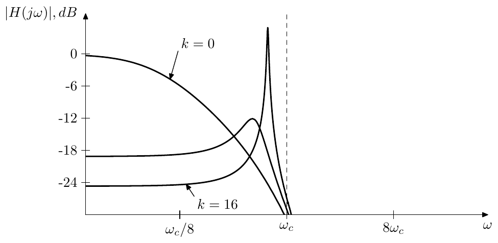
Figure 5.51: Amplitude response of the diode ladder filter for various k.
The poles of the diode ladder filter, if necessary, can be obtained by solving
which is a biquadratic equation in .
In regards to the multimode diode ladder filter, notice that the transfer functions corresponding to the outputs are different from the ones of the transistor ladder, therefore the mixing coefficients which worked for the modes of the transistor ladder filter, are not going to work the same for the diode ladder.
Resonance
In order to obtain the information about the resonating peak, we need to find frequencies at which the phase response of is or . Therefore we are interested in the solutions to the equation
Substituting for we have
The solution is not very interesting. Therefore we cancel the common factor obtaining
and therefore
Now, in order to find the selfoscillation boundary value of we need to find the frequency response of at . Substituting into (5.27) and using (5.6) we have
Now, since we are already having negative feedback in Fig. 5.48, the selfoscillation occurs at .
Note that the amplitude response in Fig. 5.51 is matching the above analysis results.
TPT model
Converting Fig. 5.48 to the instantaneous response form we obtain the structure in Fig. 5.52. From Fig. 5.52 we wish to obtain the instantaneous response of the entire diode ladder. Then we could use this response to solve the zero-delay feedback equation for the main feedback loop of Fig. 5.49.
The structure in Fig. 5.52 looks a bit complicated to solve. Of course we could always write a system of linear equations and solve it in a general way, e.g. using Gauss elimination, but this has its own complications. Therefore we would rather like to see if we somehow could still use the approach of nested zero-delay feedback loops, as we have been doing with other filters until now.
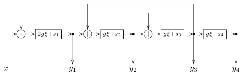
Figure 5.52: Diode ladder in the instantaneous response form.
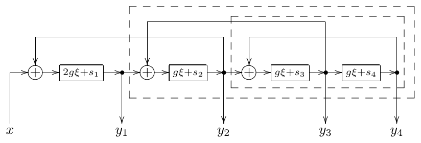
Figure 5.53: Diode ladder in the nested instantaneous response form.
Introducing the nested systems, as shown in Fig. 5.53 by dashed lines, we can first treat the innermost system which has input and outputs and . The equations for this system are
Solving for , we obtain
where and are new variables introduced as shown above. Since denote 1-pole lowpasses with halved input signals, . Respectively and thus the zero-delay feedback loop doesn’t get instantaneously unstable. The range of is
Going outside to the next nesting level we have
Solving for :
where , thus the zero-delay feedback loop doesn’t get instantaneously unstable. The range of is
Going outside to the outermost level we have
Solving for :
where , thus the zero-delay feedback loop doesn’t get instantaneously unstable. The range of is
Introducing for consistency the notation , we obtain the instantaneous response for the entire ladder
it’s not difficult to realize that
Now is the instantaneous gain of the entire diode ladder. Respectively the total gain of the of the zero-delay feedback loop in Fig. 5.49 is and thus the feedback doesn’t get instantaneously unstable provided .
Summary
The transistor ladder filter model is constructed by placing a negative feedback around a chain of four identical 1-pole lowpass filters. The feedback amount controls the resonance.
The same idea of a feedback loop around a chain of several filters also results in further filter types such as 8-pole ladder, diode ladder and SKF/TSK.
-
Quite unfortunately, there is already another class of filter structures commonly referred to as “ladder filters”. Fortunately, this class is not so widely encountered in the synth filter context, on the other hand “transistor ladder” is also a commonly used term. Therefore we’ll stick with using the term “ladder filters” for the flters based on a resonating feedback loop. ↩
-
A widely known piece of work describing this linear model is Analyzing the Moog VCF with considerations for digital implementation by T.Stilson and J.Smith. ↩
-
This time we will not develop an explicit expression for the transient response, since it’s getting too involved. Still, the general rule, which we will develop in Section 7.7, is that the transient response is always a linear combination of partials of the form (and in case of repeated poles), where are the filter poles. Respectively, as soon as some of the poles leave the left complex semiplane, the filter becomes unstable. ↩
-
As continues to grow into the unstable range, the frequencies of the exploding (or still selfoscillating, if the filter is nonlinear) sinusoidal transient response partials can change, since the imaginary part of the resonating poles can change as the poles move beyond the imaginary axis. ↩
-
We boost the input rather than the output signal for the same reason as when preferring to place the cutoff gains in front of the integrators. ↩
-
Actually, instead of we could have used the input signal for these linear combinations. However, it doesn’t matter. Since , we can express via or vice versa. It’s just that some useful linear combinations have simpler (independent of ) coefficients if rather than is being used. ↩
-
In principle, and have very similar effects. Fundamentally, they both affect the bandwidth and the resonance peak height. In Fig. 5.18 their effect on the resonance peak height is compensated, the compensation for being the gain at the output, the compensation for being embedded into the normalized bandpasses. By removing the normalization from the bandpasses we effectively introduce the gain into the feedback, and the damping thereby will control the resonance peak height too. ↩
-
Despite essentially being bandpass ladder filters, the Sallen-Key filter and its transpose can be (and are) used to deliver lowpass and highpass responses as well. ↩
-
The author has used the works of Tim Stinchcombe as the information source on the Sallen-Key filter. The idea to introduce TSK filters as a systematic concept arose from discussions with Dr. Julian Parker. ↩
-
It is easy to notice that this structure is very similar to the one of a multinotch filter with some specific dry/wet mixing ratio. ↩
-
The same structure can be obtained from a direct form II 1-pole allpass filter by the allpass substitution . It is also interesting to notice that, applying the allpass substitution principle to the structure in Fig. 5.35, we can replace the series of the two 1-pole allpass filters in Fig. 5.35 by any other allpass filter, and the modified structure will still be an allpass filter. ↩
-
In nonlinear versions of this filter this can generate a particularly complex sound, as the two resonance peaks and the input signal fight for the saturation headroom. ↩
-
One could argue that the characteristic sound of diode ladder filters is due to nonlinear behavior, however the nonlinear aspects do not show up unless the filter is driven hot enough. ↩
-
Although the denominator of is a Chebyshev polynomial, this has nothing to do with Chebyshev filters, despite the name. ↩
-
The amplitude response of can be seen in Fig. 5.51 at . ↩
-
Note that such replacement only gives a correct modal output , which is the one we usually need. Other modal outputs, if needed at all, would have to be obtained in a more complicated way by combining the output signals of the 1-poles. ↩