Chapter 4: State variable filter
After having discussed 1-pole filters, we are going to instroduce a 2-pole filter. With 2-pole filters there is more freedom in choosing the filter topology than with 1-poles, where any implementation of the latter would essentially be based on a feedback loop around an integrator. A 2-pole topology of fundamental importance and high usability is a classical analog model, commonly referred to as state-variable filter (SVF). It can also serve as a basis for building arbitrary 2-pole filters by means of modal mixture.
4.1 Analog model
The block diagram of the state-variable filter is shown in Fig. 4.1. The three outputs are the highpass, bandpass and lowpass signals. As usual, one can apply transposition to obtain a filter with highpass, bandpass and lowpass inputs (Fig. 4.2).
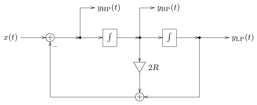
Figure 4.1: 2-pole multimode state-variable filter.
The differential equations implied by Fig. 4.1 are
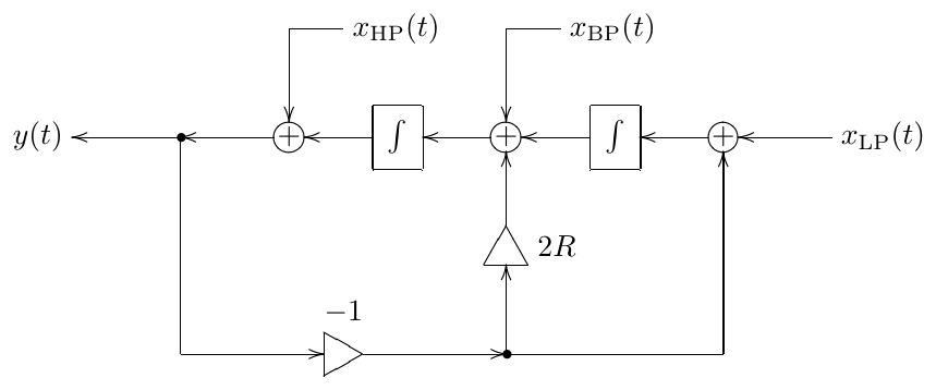
Figure 4.2: Transposed 2-pole multimode state-variable filter.
Rewriting them in terms of the lowpass signal and combining them together we obtain
or
In a similar fashion one can easily obtain the transfer functions for the output signals in Fig. 4.1. Assuming unit cutoff and complex exponential signals, we have
from where
from where
and
Thus
Notice that , that is, the input signal is split into lowpass, bandpass and highpass components. The same can be expressed in the transfer function form:
Amplitude responses
The amplitude responses of the state-variable filter are plotted in Figs. 4.3, 4.4 and 4.5. The pass-, stop- and transition bands of the low- and high-pass filters are defined in the same manner as for the 1-poles, where the transition band now can contain a peak in the amplitude response. For the bandpass the passband is located in the middle (around the cutoff), and there is a stop- and a transition band on each side of the cutoff. The slope rolloff speed is obviously -12dB/oct for the low- and high-pass, and -6dB/oct for the bandpass.
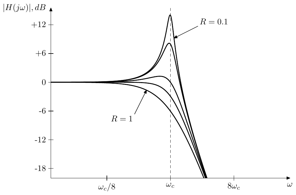
Figure 4.3: Amplitude response of a 2-pole lowpass filter.
One could observe that the highpass response is a mirrored version of the lowpass response, while the bandpass response is symmetric by itself. The symmetry between the lowpass and the highpass amplitude responses has a clear algebraic explanation: applying the LP to HP substitution to a 2-pole lowpass produces a 2-pole highpass and vice versa. The symmetry of the bandpass amplitude response has the same explanation: applying the LP to HP substitution to the 2-pole bandpass converts it into itself.
Since
the amplitude response at the cutoff is 1/2R for all three filter types. Except for the bandpass, the cutoff point is not exactly the peak location but it’s pretty close (the smaller the value of R, the closer is the true peak to ).
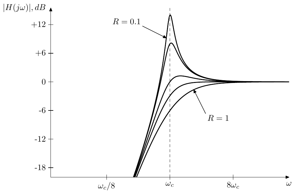
Figure 4.4: Amplitude response of a 2-pole highpass filter.
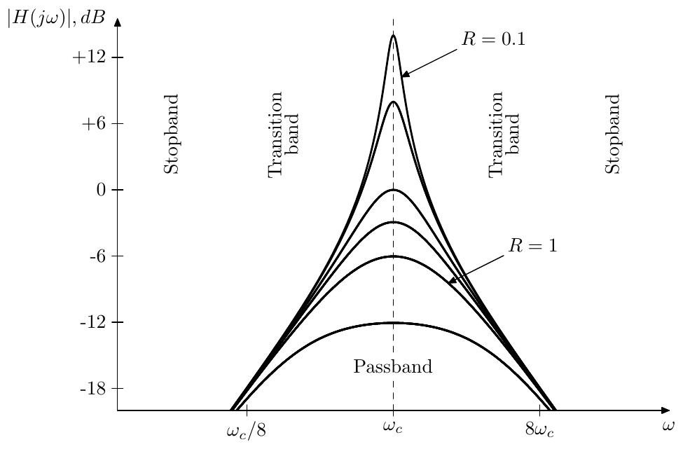
Figure 4.5: Amplitude response of a 2-pole bandpass filter.
Phase responses
The phase response of the lowpass is
where we had to switch from arctan to arccot, since the principal value of arctan gives wrong results for . Fig. 4.6 illustrates.
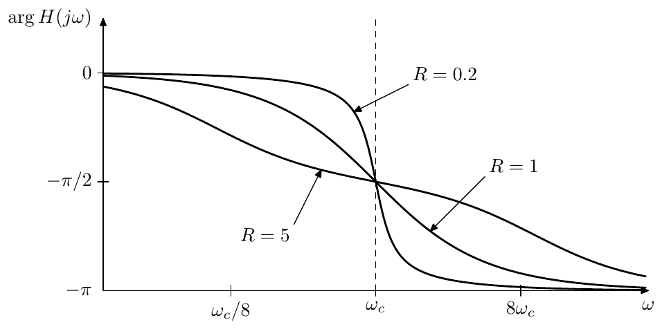
Figure 4.6: Phase response of a 2-pole lowpass filter. Bandpass and highpass responses are the same, except that they are shifted by and respectively.
We could notice the 2-pole phase response has the same kind of symmetry around the cutoff point in the logarithmic frequency scale as the 1-pole filters. This property can be explained from (4.5) by noticing that the substitution changes the sign of the argument of arccot and by using the property of arccot
We also could notice that the steepness of the phase response is affected by the parameter R. Explicitly writing the phase response in a logarithmic frequency scale we have
thus R simply scales the argument of arccot which results in stretching or shrinking of the phase response.
The bandpass phase response is a -shifted lowpass response:
The bandpass phase response is a -shifted lowpass response:
The phase response at the cutoff is for the lowpass:
respectively giving for the bandpass and for the highpass.
It can be also observed in Fig. 4.6 that the lowpass phase response is close to zero in the passband, the same as for the 1-pole lowpass. As we shuld have expected, the same also holds for the highpass’s passband. Somewhat remarkably, as we just established by evaluating the bandpass phase response at the cutoff, the same property also holds for the bandpass’s passpand, although at small values of R the phase will be close to zero only in a small neighborhood of the cutoff.
4.2 Resonance
With a 1-pole lowpass or highpass filter, the only parameter to control was the filter cutoff, shifting the amplitude response to the left or to the right in the logarithmic frequency scale. With 2-pole filters there is an additional parameter R, which, as the reader could have noticed from Figs. 4.3, 4.4 and 4.5 controls the height of the amplitude response peak occuring closely to . A narrow peak in the amplitude response is usually referred to as resonance. Thus, we can say that the R parameter controls the amount of resonance in the filter.
On the other hand, from the same figures we can notice that the resonance increases (the peak becomes higher and more narrow) as R decreases. It is easy to verify that at R = 0 the resonance peak becomes infinitely high. A little bit later we will also establish the fact that the state variable filter is stable if and only if R > 0. Thus, the parameter R actually has the function of decreasing or damping the resonance. For that reason we refer to the R parameter as the damping.1 By controlling the damping parameter we effectively control the filter’s resonance.2
Damping and selfoscillation
At R = 0 and the equation (4.3) turns into
which is effectively a spring-mass equation
or
where respectively . Starting from a non-zero initial state such system will oscillate around the origin infinitely long. Thus, in the absence of the damping signal path (Fig. 4.7), the filter will be constantly selfoscillating.3 Notably, the selfoscillation is appearing at the setting R = 0 where the resonance peak is getting infinitely high. This is a general property of resonating filters and has to do with the relationship between the filter poles and the filter’s transient response, both covered later in this chapter and additionally and in a more general form in Chapter 7.
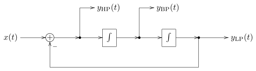
Figure 4.7: 2-pole multimode state-variable filter without the damping path (selfoscillating).
The introduction of the damping signal
reduces the amount of resonance in the filter, which in terms of a spring-mass system works as a 1st-order energy dissipation term:
This should give a better idea of why the R parameter is referred to as damping.
By further adding an external force to the spring-mass system one effectively adds the input signal.4
Resonance peak
We can find the exact position and the height of the resonance peak by looking for the local maximum of the (squared) amplitude response. E.g. for the lowpass amplitude response:
Instead of looking for the maximum of we can look for the minumum of the reciprocal function:
Clearly, is a quadratic polynomial in with the minimum at . The resonance peak position is thus
where for (we are considering only positive values of R) there is no minimum at and respectively no resonance peak. Note that the peak thereby starts at at and, as R decreases to zero, moves towards .
The resonance peak height is simply the value of the amplitude response evaluated at :
and
Thus at the peak height is formally , corresponding to the amplitude response not having the peak yet. At we have . The above expression also allows us to find the value of R given a desired peak height A. Starting from
we have
Taking into account the allowed range of R (which is ), we obtain
Recalling that the amplitude response of the 2-pole highpass is simply a symmetrically flipped amplitude response of the 2-pole lowpass, we realize that the same considerations apply to the 2-pole highpass, except that the expression for needs to be reciprocated. For the bandpass filter the amplitude response peak is always exactly at the cutoff.
Butterworth filter
The threshold value at which the resonance peak starts to appear has another interesting property. At this setting the (logarithmic frequency scale) amplitude responses of the 2-pole lowpass and highpass are shrunk horizontally two times around the cutoff point, as compared to those of 1-poles (the phase response is transformed in a more complicated way, which is of little interest to us here). This is a particular case of a Butterworth filter. Butterworth filters will be discussed in a generalized form in Chapter 8, but we can also show this shrinking property explicitly here. Indeed, for we have
Now, the substitution corresponds to the two times shrinking in the logarithmic frequency scale: . Thus, for the lowpass 2-pole we have
and for the highpass filter we have
The readers can refer to Fig. 8.13 for the illustration of the shrinking effect. Since for the amplitude response obtains a resonance peak, the Butterworth 2-pole filter is the one with the “sharpest” possible cutoff among all non-resonating 2-poles.
4.3 Poles
Solving we obtain the poles of the filter at
Thus, the poles are located in the left semiplane if and only if R > 0. As with 1-poles, the location of the poles in the left semiplane is sufficient and necessary for the filter to be stable.5
For the poles are located on the unit circle
This also implies that R is equal to the cosine of the angle between the negative real axis and the direction to the pole (Fig. 4.8).
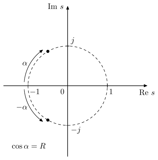
Figure 4.8: Poles of a resonating 2-pole filter ().
As R is getting close to zero, the poles are getting close to the imaginary axis. By definition of a pole, the transfer function is infinitely large at the poles, which means it is also having large values on the imaginary axis close to the poles. This corresponds to the resonance peak appearing in the amplitude response. At R = 0 the poles are located right on the imaginary axis and the filter selfoscillates.
At the poles are real and mutually reciprocal:6
(Fig. 4.9). The filter thus “falls apart” into a serial combination of two 1-pole filters:
where .7 These 1-pole filters become visible in the amplitude responses at sufficiently large as two different “cutoff points” (Fig. 4.10).
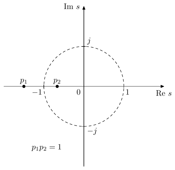
Figure 4.9: Poles of a non-resonating 2-pole filter ().
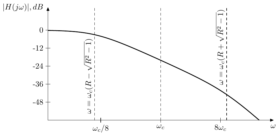
Figure 4.10: Amplitude response of a non-resonating 2-pole lowpass filter.
Resonance redefined
The pole positions can give us another way of defining the point where we consider the resonance to appear. Previously we have found that the resonance peak appears at . However, the amplitude response peak is only one manifestation of the resonance effect. Another aspect of resonance is that, as we shall see later, the transient response of the filter contains sinusoidal oscillation, which occurs whenever the poles are complex. Therefore, using the presence of transient oscillations as the alternative definition of the resonance, we can say that the resonance occurs when .
Similarly to , the threshold setting has a special property. At this setting both poles are located at and the transfer function of the 2-pole lowpass becomes equal to the transfer function of two serially connected 1-pole lowpasses:
while the transfer function of the 2-pole highpass becomes equal to the transfer function of two serially connected 1-pole highpasses:
This means that at this value of the (decibel-scale) amplitude responses of the 2-pole lowpass and highpass are stretched vertically two times compared to those of the 1-pole lowpass and highpass (Fig. 4.11), and the same holds for the phase responses (Fig. 4.12).
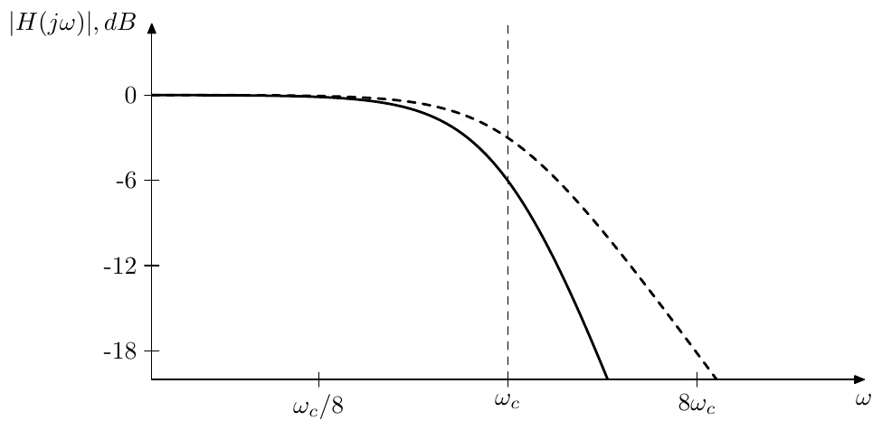
Figure 4.11: Amplitude response of the 2-pole lowpass filter at (solid line) compared to the amplitude response of the 1-pole lowpass filter (dashed line).
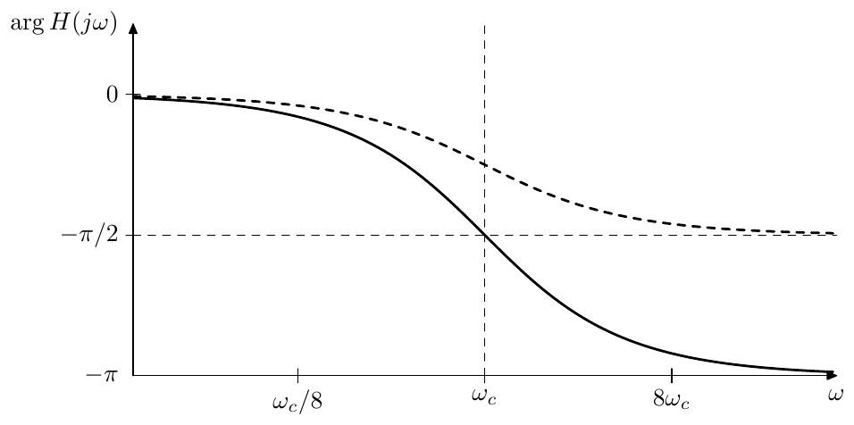
Figure 4.12: Phase response of the 2-pole lowpass filter at (solid line) compared to the amplitude response of the 1-pole lowpass filter (dashed line).
Non-unit cutoff
If then the transfer function denominator becomes (or , if no simplifications are performed on the entire transfer function) and the formula for the poles becomes
The formula (4.9) can be obtained either by directly solving the quadratic equation or by noticing that the cutoff substitution scales the poles according to . Complex poles are therefore located on the circle of radius (Fig. 4.13), while real poles have a geometric mean equal to (Fig. 4.14).
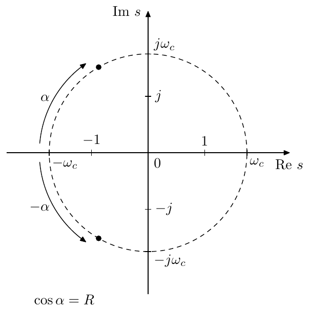
Figure 4.13: Poles of a resonating 2-pole filter ().
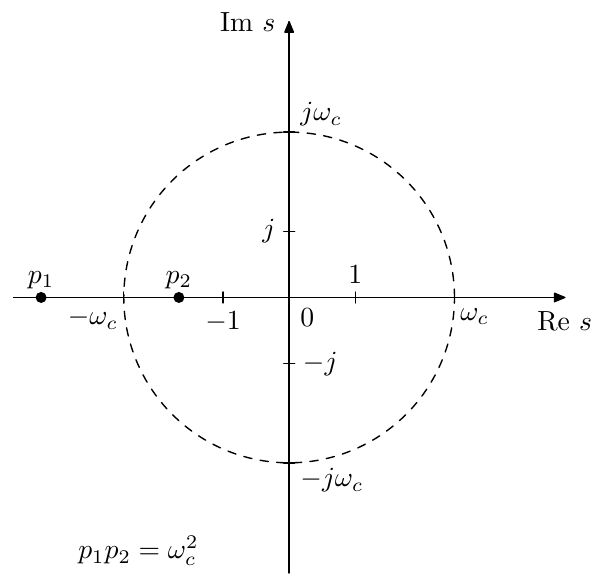
Figure 4.14: Poles of a non-resonating 2-pole filter ().
Transfer function in terms of poles
Writing the lowpass transfer funtion in terms of poles we have for
and for an arbitrary respectively
Respectively
from where
In terms of and the same turns into
and
Notice that thereby is a geometric mean of the 1-pole cutoffs, and is a ratio of their arithmetic and geometric means. Equations (4.12) can be used to represent a series of two 1-poles with given cutoffs by an SVF.8
Pole cutoff and damping
A pair of complex poles of an SVF must be a conjugate pair, therefore we have , and . The equations (4.10) in this case turn into
These relationships motivate the introduction of the notion of the “associated cutoff and damping” of an arbitrary pair of conjugate poles and , where we would have
and
(Fig. 4.13 can serve as an illustration).
This idea is particularly convenient, if we imply that a particular high-order transfer function is to be implemented as a cascade of 2-poles (further discussed in Section 8.2), in which case (4.13) gives us ready formulas for the computation of the cutoff and damping of the respective 2-pole. Also, unless the high-order transfer function is having coinciding complex poles, the separation of complex poles into pairs of conjugate poles is unambiguous.
The same can be done for real poles, if desired, where we can use (4.11) instead of (4.13) but this would work only under the restriction that both poles are having the same sign (Fig. 4.14 can serve as an illustration).9 Also the grouping of such poles into pairs can be done in different ways.
Sometimes the same terminology is also convenient for zeros. Even though formally it is not correct, since zeros are not directly associated with a cutoff or damping, it is sometimes handy to treat a pair of zeros as roots of a polynomial .
4.4 Digital model
Skipping the naive implementation, which the readers should be perfectly capable of creating and analyzing themselves by now, we proceed with the discussion of the TPT model.
Assuming instantaneous responses for the two trapezoidal integrators one can redraw Fig. 4.1 to obtain the discrete-time model in Fig. 4.15.
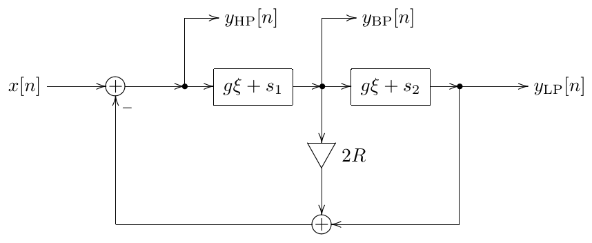
Figure 4.15: TPT 2-pole multimode state-variable filter in the instantaneous response form.
Picking as the zero-delay feedback equation’s unknown10 we obtain from Fig. 4.15:
from where
from where
Apparently (4.14) has the form (3.37), where the total instantaneous gain of the zero-delay feedback loop in Fig. 4.15 is and thus the instantaneously unstable case occurs when the denominator of (4.14) is negative. However, as long as and , the denominator of (4.14) is always positive:
thus under these conditions the filter in not becoming instantaneously unstable.
Using we can proceed defining the remaining signals in the structure, in the same way as we did for the 1-pole in Section 3.9. Assuming that we are using trasposed direct form II integrators (Fig. 3.11), are the states of the elements in the respective integrators and (prewarped). Therefore by precomputing the values and in advance, the formula (4.14) can be computed in 2 subtractions and 2 multiplications. What remains is the processing of both integrators. A transposed direct form II integrator can be computed in 1 multiplication and 2 additons. Thus, the entire SVF processing routine needs 4 multiplications and 6 additions/subtractions:
// perform one sample tick of the SVF
HP := (x-g1*s1-s2)*d; // g1=2R+g, d=1/(1+2Rg+g^2)
v1 := g*HP; BP := v1+s1; s1 := BP+v1; // first integrator
v2 := g*BP; LP := v2+s2; s2 := LP+v2; // second integrator
If we are not interested in the highpass signal, we could obtain a more optimal implementation by solving for instead:
This gives us:
// perform one sample tick of the SVF BP/LP
BP := (g*(x-s2)+s1)*d; // d=1/(1+2Rg+g^2)
v1 := BP-s1; s1 := BP+v1; // first integrator
v2 := g*BP; LP := v2+s2; s2 := LP+v2; // second integrator
This implementation has 3 multiplications and 6 additions/subtractions.
If we need only the BP signal, then we could further transform the expressions used to update the integrators:
// perform one sample tick of the SVF BP
BP := (g*(x-s2)+s1)*d; // d=1/(1+2Rg+g^2)
BP2 := BP+BP; s1 := BP2-s1; // first integrator
v22 := g*BP2; s2 := s2+v22; // second integrator
That’s 3 multiplications and 5 additions/subtractions.
4.5 Normalized bandpass filter
By multiplying the bandpass filter’s output by :
we obtain a bandpass filter which has a unit gain (and zero phase response) at the cutoff:
For that reason this version of the 2-pole bandpass filter is referred to as a unit-gain or normalized bandpass. Fig. 4.16 illustrates the amplitude response.
The normalized bandpass has a better defined passband than the ordinary bandpass, since here we can define the frequency range where as the passband. Notably, in Fig. 4.16 one observes that the width of the passband grows with . At the same time from Fig. 4.6 one can notice that the width of the band where the bandpass phase response is close to zero also grows with . Thus, the phase response of the normalized bandpass filter is close to zero in the entire passband of the filter, regardless of .11
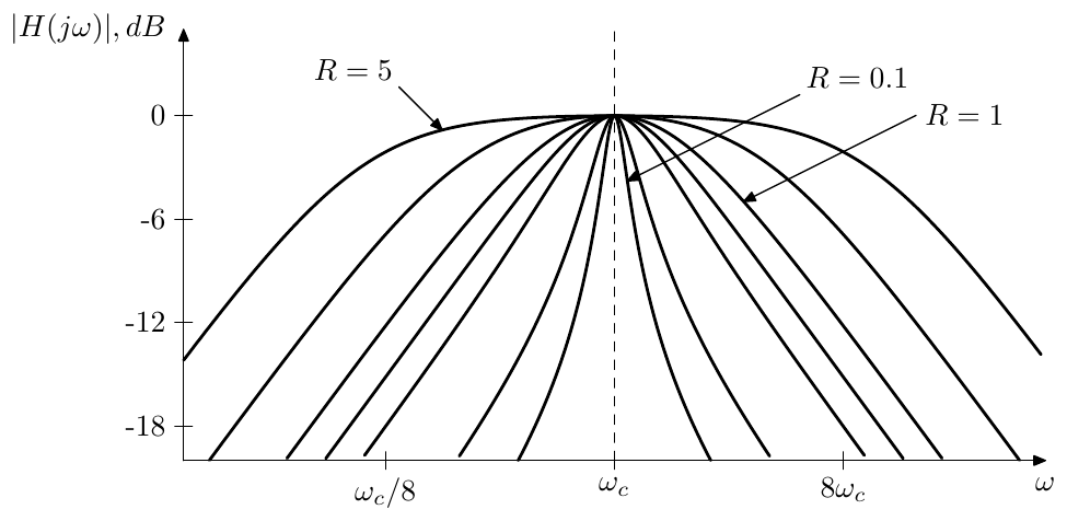
Figure 4.16: Amplitude response of a 2-pole unit gain bandpass filter.
Rewriting (4.4) in terms of the normalized bandpass we get
that is
Topology
Notice that the unit gain bandpass signal can be directly picked up at the output of the gain element as shown in Fig. 4.17.
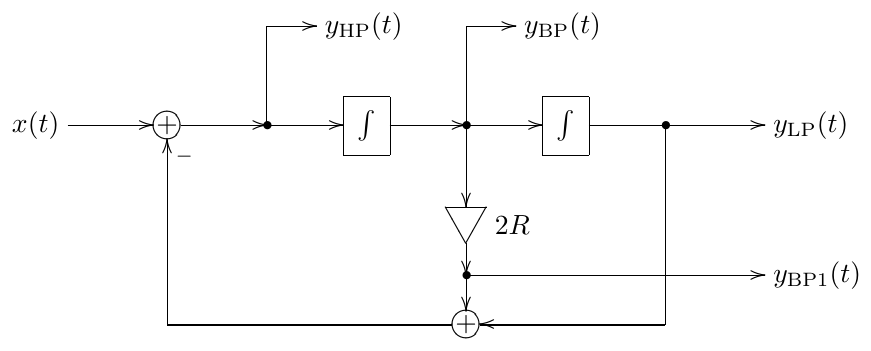
Figure 4.17: State-variable filter with a normalized bandpass output.
If the damping parameter is to be modulated at high rate, rather than multiplying the bandpass output by , it might be better to multiply the filter’s input by :
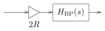
The reasoning is pretty much the same as for positioning the cutoff gains before the integrators or for preferring the transposed (multi-input) filters for modal mixing: we let the integrator smooth the jumps or quick changes in the signal. This will be given for granted if we use the transposed version of Fig. 4.17.
Instead of using the transposed version, we could inject the input signal into the Fig. 4.17 filter structure as shown in Fig. 4.18. However, by multplying the input rather than the output by we have not only changed the “BP” output signal to normalized bandpass, we have also changed the amplitudes of the LP and HP outputs. Notably, Fig. 4.18 is essentially the transposed version of Fig. 4.17, except for the relative placement of the second integrator and an invertor.
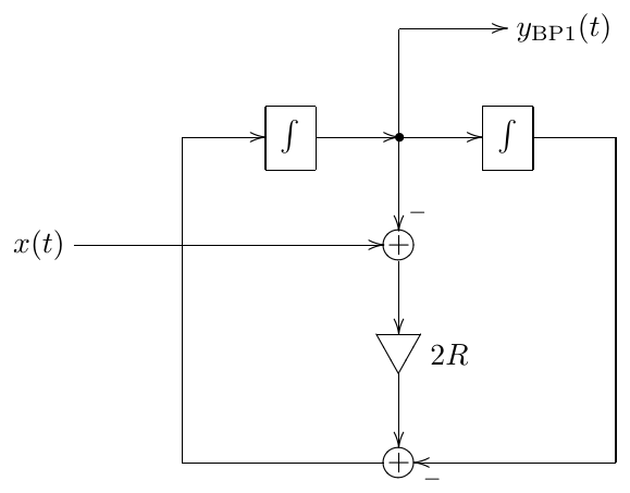
Figure 4.18: Normalized bandpass state-variable filter with prefilter gain.
Prewarping
The standard application of the bilinear transform prewarping technique implies that we want the cutoff point to be positioned exactly at on the digital frequency axis. However with the normalized bandpass filter the positioning of the left and right transition band slopes is more important than the exact positioning of the cutoff. At the same time, the damping parameter doesn’t seem to have much (or any) vertical effect on the amplitude response, mainly controlling the distance between the slopes. Thus we have two degrees of control freedom (the cutoff and the damping) which we could attempt to use to position the two slopes as exactly as possible. Instead of developing the corresponding math just for the normalized bandpass filter, though, we are going to do this in a more general manner in Section 4.6.
4.6 LP to BP/BS substitutions
The 2-pole unit gain bandpass response can be obtained from the lowpass response by the so-called LP to BP (lowpass to bandpass) substitution:
We will also occasionally refer to the LP to BP substitution as the LP to BP transformation, making no particular disctinction between both terms.
Since and are used symmetrically within the right-hand side of (4.16), it immediately follows that the result of the substitution is invariant relative to the LP to HP substitution . Therefore the result of the LP to BP substitution has an amplitude response which is symmetric in the logarithmic frequency scale.
Using , we obtain
or
Denoting the new as we write
Instead of trying to understand the mapping of to it is easier to understand the inverse mapping from to , as explicitly specified by (4.17). Furthermore, it is more illustrative to express in the logarithmic scale:
Thus
Since takes up the entire real range of values in each of the cases and and respectively, so does ,
This means that the entire range is mapped once onto the positive frequencies and once onto the negative frequencies . Furthermore, the mapping and its inverse are strictly increasing on each of the two segments and , since . The unit frequencies are mapped from .
Since we are often dealing with unit-cutoff transfer functions (), it’s interesting to see to which frequencies the unit cutoff is mapped. Recalling that the entire bipolar range of is mapped to the positive range of , we need to include the negative cutoff point () into our transformation. On the other hand, we are interested only in positive , since the negative-frequency range of the amplitude response is symmetric to the positive-frequency range anyway. Under these reservations, from (4.18) we have:
from where , or, changing the logarithm base:
Note that the above immediately implies that the two points are located at mutually reciprocal positions.
The distance in octaves between the two points can be defined as the bandwidth of the transformation:
Since the points are mutually reciprocal, they are located at octaves from .
Inverting (4.19) we can obtain the damping, given the bandwidth :
Frequency axis warping and parameter prewarping
An important consequence of the fact that the LP to BP substitution can be seen as a mapping of the axis is that the only effect of the variation of the parameter is the warping of the frequency axis. This means that (like in the bilinear transform) the amplitude and phase responses are warped identically and the relationship between amplitude and phase responses is therefore preserved across the entire range of .
If LP to BP substitution is involved, the resulting frequency response has two points of interest which are the images of the original point at , which often is the cutoff point of the original frequency response.12 Given a digital implementation of such LP to BP substitution’s result, we can prewarp the parameter of the substitution in such a way that the distance between the points in the digital frequency response is identical to the distance between those in analog frequency response.
Indeed, given the original value of , we can use (4.19) to compute the distance between the points. We know that the points are positioned at octaves from , or, if the substitution result has its own cutoff parameter, from . That is
So, these are the frequencies at which the unit frequency’s image points would be normally located on an analog filter’s response and where we want them to be located on the digital filter’s response. If are the points on the digital frequency response, then by (3.10) the corresponding analog points should be located at
At unit cutoff the points would have been mutually reciprocal. If the cutoff is not unity, then it must be equal to the geometric mean of :
while the bandwidth is simply the logarithm of the ratio of :
Given , we obtain from (4.20).
So, we have obtained the prewarped parameters and , which can be used to control a bilinear transform-based digital implementation of an LP to BP substitution’s result, thereby ensuring the correct positioning of the points. Particularly, treating the normalized bandpass filter as the result of LP to BP substitution’s application to a 1-pole lowpass , we could prewarp the bandpass filter’s parameters to have exact positioning of the -3dB points on the left and right slopes (since these are the images of the 1-pole lowpass’s unit cutoff point).
In principle, any other two points could have been chosen as prewarping points, where the math is much easier if these two points are located symmetrically relatively to the cutoff in the logarithm frequency scale. We will not go into further detail of this, as the basic ideas of deriving the respective equations are exactly the same.
Poles and stability
The transformation of the poles and zeros by the LP to BP transformation can be obtained from
resulting in
Regarding the stability preservation consider that the sum in (4.21) is located in the same complex semiplane (left or right) as . Therefore, as long as , the original value is located in the same semiplane as its images . which implies that the stability is preserved. On the other hand, negative values of “flip” the stability.
Topological LP to BP substitution
As for performing the LP to BP substitution in a block diagram, differently from the LP to HP substitution, here we don’t need differentiators. The substitution can be performed by replacing all (unit-cutoff) integrators in the system with the structure in Fig. 4.19, thereby substituting for , which is algebraically equivalent to (4.16).13
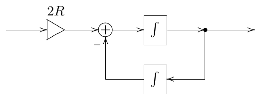
Figure 4.19: “LP to BP” integrator.
LP to BS substitution
The LP to BS (lowpass to bandstop) substitution14 is obtained as a series of LP to HP substitution followed by an LP to BP substitution. Indeed, applying the LP to BP substitution to a 1-pole highpass, we obtain the 2-pole notch (“bandstop”) filter. Therefore, applying a series of LP to HP and LP to BP substitutions to a 1-pole lowpass we also obtain the 2-pole notch filter.
Combining the LP to HP and LP to BP substitutions expressions in the mentioned order gives an algebraic expression for the LP to BS substitution:
The bandwidth considerations of the LP to BS substitution are pretty much equivalent to those of LP to BP substitution and can be obtained by considering the LP to BS substitution as an LP to BP substitution applied to a result of the LP to HP substitution.
The block-diagram form of the LP to BS substitution can be obtained by directly implementing the right-hand expression in (4.22) as a replacement for the integrators. This however requires a differentiator for the implementation of the term of the sum.
4.7 Further filter types
By mixing the lowpass, bandpass and highpass outputs one can obtain further filter types. We are now going to discuss some of them.
Often it will be convenient to also include the input signal and the normalized bandpass signal into the set of the mixing sources. Apparently this doesn’t bring any new possibilities in terms of the obtained transfer functions, since the input signal can be obtained as a linear combination of LP, BP and HP signals. However the mixing coefficients might look simpler in certain cases. One can also go further and consider using different topologies implementing a given 2-pole transfer function. Such topologies could differ not only in which specific signals are mixed, but also whether certain mixing coefficients are used at the input or at the output, whether transposed or non-transposed SVF is being used, etc. We won’t go here into addressing this kind of detail, however the discussion of the topological aspects of the normalized bandpass in Section 4.5 could serve as an example.
Band-shelving filter
By adding/subtracting the unit gain bandpass signal to/from the input signal one obtains the band-shelving filter (Fig. 4.20):
As with 1-pole shelving we can also specify the shelving boost in decibel:
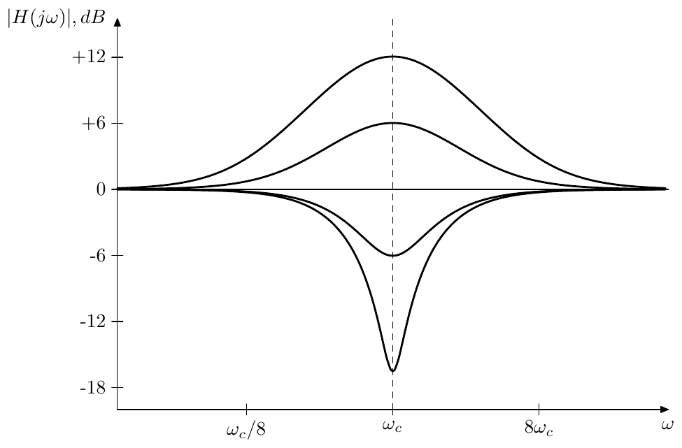
Figure 4.20: Amplitude response of a 2-pole band-shelving filter for and varying .
The immediately noticeable problem in Fig. 4.20 is that the bandwidth of the filter varies with the shelving boost . A way to address this issue will be described in Chapter 10.
Low- and high-shelving filters
Attempting to obtain 2-pole low- and high-shelving filters in a straightforward fashion:
we notice that the amplitude responses of such filters have a strange dip (for ) or peak (for ) even at a non-resonating setting of (Fig. 4.21). This peak/dip is due to a steeper phase response curve of the 2-pole lowpass and highpass filters compared to 1-poles. A way to build 2-pole low- and high-shelving filters, which do not have this problem, is described in Chapter 10.
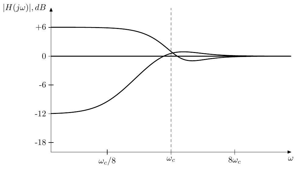
Figure 4.21: Amplitude response of a naive 2-pole low-shelving filter for and varying .
Notch filter
At the band-shelving filter turns into a notch (or bandstop) filter (Fig. 4.22):
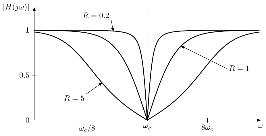
Figure 4.22: Amplitude response of a 2-pole notch filter. The amplitude scale is linear.
Allpass filter
At the band-shelving filter turns into an allpass filter (Fig. 4.23):
It is not difficult to show that for purely imaginary the absolute magnitudes of the transfer function’s numerator and denominator are equal and thus .
We could also notice that the phase respose of the 2-pole allpass is simply the doubled 2-pole lowpass phase response:
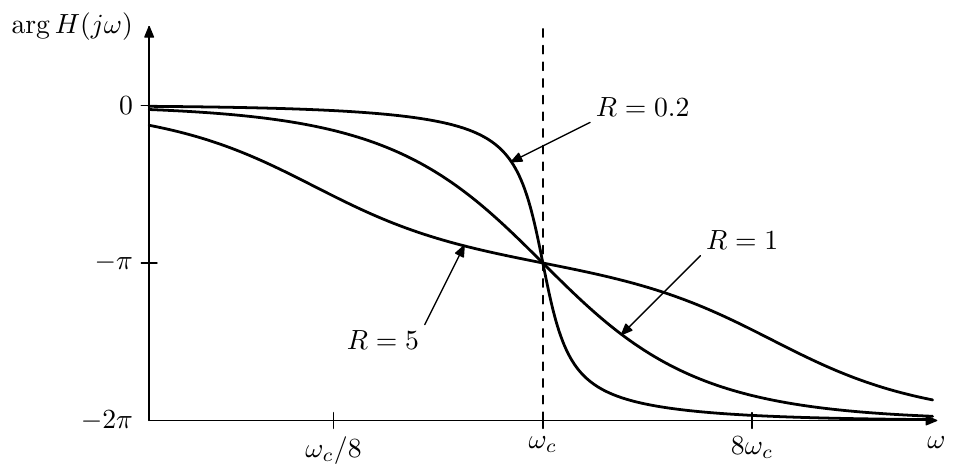
Figure 4.23: Phase response of a 2-pole allpass filter.
Thus the allpass phase response has the same symmetry around the cutoff point and the damping parameter has a similar effect on the phase response slope.
At the 2-pole allpass can be decomposed into the product of 1-pole allpasses:
where . At we have and the filter turns into the squared 1-pole allpass:
Peaking filter
By subtracting the highpass signal from the lowpass signal (or also vice versa) we obtain the peaking filter (Fig. 4.24):
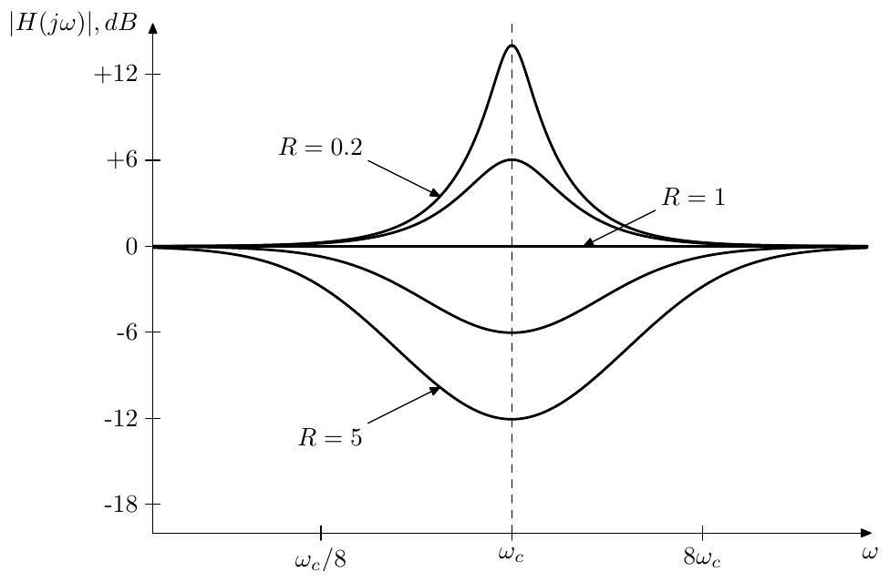
Figure 4.24: Amplitude response of a 2-pole peaking filter.
The peaking filter is a special kind of bandshelving filter. However, as one can see from Fig. 4.24, the bandwidth of the filter varies drastically with , which often may be undesired. A “properly built” bandshelving filter allows to avoid this problem. This topic is further discussed in Chapter 10.
Arbitrary 2-pole transfer functions
It’s easy to see that the state-variable filter can be used to implement any 2nd-order stable differential filter. Indeed, consider the generic 2nd-order transfer function
where we assume .15 Then
where we introduced and .
4.8 Transient response
In the transient response analysis of the state-variable filter we will concentrate on the lowpass output. The bandpass and highpass can be obtained from the lowpass using (4.1):
Using (4.10) we rewrite (4.3) in terms of poles, obtaining
where . Let16
Therefore
and
Noticing that the last expression is simply the doubled left-hand side of (4.26) we obtain an equivalent form of (4.26):
Splitting the latter in two halves we have:
Adding both equations (4.30) back together, we obtain (4.29), which is equivalent to (4.26). This means that if and are solutions of (4.30) then using (4.27) we can find from and , which will be the solution of (4.26).
Now, each of the equations (4.30) is a Jordan 1-pole with input signal . Applying (2.22) we obtain
or, for , we have from (2.23):
where
and where and denote the steady-state and transient response parts of respectively. Expressing via from (4.27) we have
For the steady-state response we therefore obtain from (4.31):
where
is the familiar 2-pole lowpass transfer function. The steady-state response is therefore having the same form for a complex exponential as in case of the 1-pole filter. For signals of general form we respectively obtain the same formula (2.20a) as for 1-poles.
For the transient response we have
where we introduce the ordinary (except that may be complex) 1-pole lowpass transfer functions
Provided we are having a sum of two exponentially decaying terms. Since , the initial value of this sum is , the same as in the 1-pole case, so we’re having an exponentially decaying discrepancy between the output signal and the steady-state response. However the decaying is now being “distributed” between two exponents and . Also notice that while in the 1-pole case the decaying was only affected by the initial state , in the 2-pole case is also a part of the initial state and therefore also affects the decaying shape. Apparently, is the state of the second (“lowpass”) integrator of the SVF, while, according to (4.25a), is essentially the state of the first (“bandpass”) integrator.
At the transient response grows infinitely and the filter explodes.
Steady-state response
In regards to the choice of the steady-state response, there is a similar ambiguity arising out of evaluating the inverse Laplace transform of to the left or to the right of the poles of . We won’t specifically go into the analysis of this situation for the real poles occurring in the case . Complex poles occurring in the case deserve some specical attention.
Apparently in this case, and we wish to know how much does the inverse Laplace transform change when we switch the integration path from to . By the residue theorem this change will be equal to the sum of the residues of at and respectively, which is
(where we have used (4.33)). That is we are again obtaining the terms which already exist in the transient response and the integration path choice only affects the amplitudes of the transient response partials, as long as we are staying within the region of convergence of .
The case of coinciding poles requires a separate analysis which can be done as a limiting case . The respective discussion is occurring later in this section. Even though we don’t specifically address the question of evaluation of the inverse Laplace transform in the steady-state response there, it should be clear what the principles would be.
Continuity
Since the input signal of an SVF passes through two integrators on the way to the lowpass output, the lowpass signal should not only always be continuous but should also always have a continuous 1st derivative. Therefore the appearance of besides in the transient response expression must have somehow taken care of that. Let’s verify that this is indeed the case.
Evaluating (4.34) at using we obtain
where we have used (4.33). Evaluating the derivative of (4.34) at we obtain
which confirms our expectations.
Complex vs. real poles
If are complex we have
The mutual conjugate property of poles will ensure that the two terms of (4.34) are mutually conjugate as well, therefore the addition result is purely real and has the form
The transient response therefore is a sinusoidal oscillation of frequency decaying (or exploding) as . Fig. 4.25 illustrates.
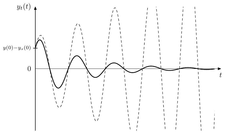
Figure 4.25: Transient response of a resonating 2-pole lowpass filter (dashed line depicts the unstable case).
For purely real poles the transient response contains just two real exponents of the form , thereby having no oscillations. However, it can still contain one “swing” at certain combinations of the amplitudes of the transient partials and (Fig. 4.26).
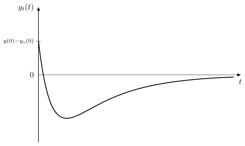
Figure 4.26: Transient response of a non-resonating 1-pole lowpass filter (for the case of a single zero-crossing).
Strong resonance case
The decay speed of the transient response oscillation (4.36) gets slower as decreases, which leads to an increased perceived duration of the transient in the output signal. Therefore at high resonance settings a transient in the input signal will produce audible ringing at resonance frequency, even if the steady-state signal doesn’t contain it.
A pretty characteristic and easy to analyse case occurs if we suddenly switch off the filter’s input signal. At this moment the steady-state response instantaneously turns to zero and (4.34) turns into
Therefore
Unless both and , the signal will have a non-zero amplitude and according to (4.36) we are having a sinusoid of frequency decaying as .
The opposite situation of a signal being turned on is a kind of a dual case of turning a signal off. Indeed, let be some infinitely long (that is ) steady input signal and let be the respective output signal. Assuming that the filter is stable and that the initial time moment was at , by any finite time moment the transient response component of has decayed to zero, and consists solely of the steady-state response. Let
be another infinitely long signal decribing the case of the signal being turned off and let be the respective output signal. The signal contains a transient at , thus contains a non-zero transient response component for . The case of being turned on is respectively described by
and we let denote the corresponding output signal. Since the system is linear, the output signals are related in the same way as the input signals:
However doesn’t contain any transient response, therefore the only transient response present in is coming from , simply having the opposite sign.
The effect of the transient response is particularly remarkable if the input signal is a sinusoid of the same frequency as the transient response. First considering the case of turning such sinusoid off we take
We must have the same sinusoid at the output:
where the transient response’s amplitude and phase and may differ from the steady-state response’s and due to the additional factor appearing in the signal. However from the requirement of continuity of and at we may conclude that and for .
Now let’s consider the case of turning the signal on. We let . Since we already know that for , we are interested only in for where we have
Since at we have and , we may in this case rewrite the above as
That is the sinusoid in the output signal is exponentially fading in as . Effectively the transient response is suppressing the steady state signal in the beginning and then slowly lets it fade in (Fig. 4.27).
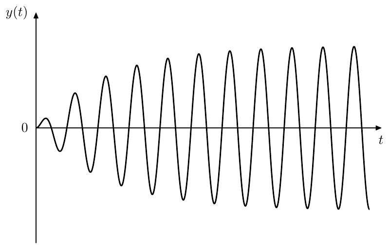
Figure 4.27: Initial suppression of the steady-state signal at by the transient response.
Selfoscillation
At the transient response oscillates at a constant amplitude, the frequency of the oscillation being and coinciding with the infinitely high peak of the amplitude response. Thus, if in the absence of the input signal the system is somehow in a non-zero state, it will stay in this state forever, producing a sinusoid of frequency . Such state of oscillating without an input signal is referred to as selfoscillation.
At the transient response turns into an infinitely growing signal, while the oscillation frequency becomes lower than according to (4.36). In nonlinear filters at the growing amplitude of the oscillating transient response will be limited by the saturation, which thereby prevents the filter from exploding. In either case, apparently it is the transient response which is responsible for the selfoscillation of the filter.
We can therefore refer to as the selfoscillation range of the filter. The boundary at which the selfoscillation appears may be referred to as selfoscillation point.17
At the selfoscillation point the poles of the system are located right on the imaginary axis and we can “hit” them with an input sinusoidal signal of frequency . Since , the steady-state response becomes infinite too and we need a different choice of the steady-state response signal.
A real sinusoidal signal of frequency consists of two complex sinusoidal signals of frequencies . Each of these two signals hits the respective complex pole of the system at . As we should recall from the discussion in Section 2.15, when a system pole is hit by an input , the output of the system consists of a linear combination of partials and , where we cannot unambiguously select the steady-state response part. From two conjugate poles and we’ll get a linear combination of and and another one of and . After these signals are further combined by (4.32) we’ll get a real signal of the form
Thus, the output signal is a sinusoid of frequency with the amplitude asymptotically growing as a linear function of time.18 Clearly, this is a marginal case between the sinusoidal output stabilizing with time if , as e.g. shown in Fig. 4.27, and exponentially exploding if .
Coinciding poles
A special situation occurs if and thus . The denominator therefore turns to zero, but we can treat this as a limiting case of . Let (where and ). Noticing that
we can replace in (4.34) with before taking the limit:
In the first term of (4.37) we have
and in the second term respectively
and (4.37) at can be rewritten as
Thus, in the case of the terms contained in the transient response are having the form or .
The change (4.35) in the inverse Laplace transform in the steady-state response as we take the integral to the left or to the right of the poles of respectively becomes
where we have used l’Hôpital’s rule.19 Thus, the change is again solely in the amplitudes of the transient response partials.
It is important to realize that the different form of the transient response components at doesn’t imply that the filter behavior is abruptly switched at this point. The switching of the mathematical expression is solely due to the limitations of the mathematical notation, but doesn’t correspond to a jump in any of the signals.
The same result could have been obtained formally by introducing the helper variables and differently:20
(where ) thereby obtaining the equations
which can be solved using 1-pole techniques. Since is the input signal for we have a serial connection of 1-poles, building up a Jordan chain. As we should remember from the discussion of Jordan chains in Section 2.15, the transient response will consist of the partials of the form and . However, due to a completely different substitution of variables, we wouldn’t have known, whether the output is changing in a continuous way as crosses the point . On the other hand, obtaining the result as a limiting case, as we did earlier, gives an answer to that question.
Bandpass and highpass
Notice that (4.25) can be applied separately to steady-state and transient responses (in the sense that the results will still give correct separation of the signal into the steady-state and transient parts). Indeed, e.g. applying (4.25a) to a complex exponential we obtain
which matches . Therefore , when applied to a lowpass steady-state response , will give bandpass steady-state response, etc.
This means that the transient response for the bandpass and highpass signals can be obtained by differentiating the lowpass transient response according to (4.25), resulting in a sum of the same kind of exponential terms and (or and in case ). We won’t write the resulting expressions explicitly here.
Summary
The state-variable filter has the structure shown in Fig. 4.1. Contrarily to the ladder filter, the resonance strength in the SVF is controlled by controlling the damping signal. The multimode outputs have the transfer functions
and can be combined to build further filter types.
-
A more correct term, used in theory of harmonic oscillations, is damping ratio, where the commonly used notation for the same parameter is . ↩
-
The “resonance” control for the SVF filter can be introduced in a number of different ways. One common approach is to use the parameter , however this doesn’t allow to go easily into the selfoscillation range in the nonlinear versions of this filter, also the math is generally more elegant in terms of R than in terms of Q. Another option is using , which differs from the resonance control parameter of SKF/TSK filters (discussed in Section 5.8) just by a factor of 2, the selfoscillation occuring at . Other, more sophisticated mappings, can be used for a “more natural feel” of the resonance control. ↩
-
The selfoscillating state at R = 0 is a marginally stable state. As mentioned earlier, due to the noise present in the system (such as numerical errors in a digital implementation), we shouldn’t expect to be able to exactly hold a system in a marginally stable state. In order to have reliable selfoscillation one usually needs to introduce nonlinear elements into the system. E.g. by introducing the saturating behavior one would be able to lower R below 0, thereby increasing the resonance even further, without making the filter explode. So, while selfoscillation formally appears at R = 0, it is becoming reliable at R < 0, given that nonlinearities prevent the filter from exploding. ↩
-
Thereby the differential equation becomes formally equivalent to an SVF, but there still is an essential difference. The state of a spring-mass system consists of a position and a velocity . Changes to the system parameters will therefore directly change the kinetic and potential energies, which can result in a sudden increase or reduction of the amplitude of the swinging. In comparison, in the SVF the system state consists of the “lowpass” integrator’s state and “bandpass” integrator’s state, which according to (4.1) is . In this case changes to the filter parameters will affect the filter’s output in a more gradual way. Particulary, according to (2.29), changes to the cutoff will not affect the output amplitude at all. ↩
-
Later we will discuss the transient response of the SVF and the respective effects of the poles position on the stability. ↩
-
Actually, the poles are mutually reciprocal at any R (since their product should be equal to the constant term of the denominator). For complex poles the reciprocal property manifests itself as conjugate symmetry of the poles, since the poles are lying on the unit circle and the reciprocation does not change their absolute magnitude. ↩
-
Of course the same decomposition is formally possible for complex poles, but a 1-pole filter with a complex pole cannot be implemented as a real system. ↩
-
Apparently, (4.12) defines only the denominator of the SVF’s transfer function. The numerator would need to be computed separately. ↩
-
Apparently (4.11) can be used all the time, regardless of whether the poles are complex or real. It’s just that in case of complex poles we have simpler and more intuitive formulas (4.13). ↩
-
The state-variable filter has two feedback paths sharing a common path segment. In order to obtain a single feedback equation rather than an equation system we should pick a signal on this common path as the unknown variable. ↩
-
This can be confirmed in a more rigorous manner by the fact (which we establish in Section 4.6) that the frequency response of the 2-pole normalized bandpass filter can be obtained from the frequency response of the 1-pole lowpass filter by a frequency axis mapping. ↩
-
We are using and instead of previously used and notation for the respective point, since we are going to need to denote the substitution result’s cutoff. ↩
-
For a differentiator, a similar substitution structure (containing an integrator and a differentiator) is trivially obtained from the right-hand side of (4.16). ↩
-
Notice that BS here stands for “bandstop” and not for “band-shelving”. The alternative name for the substitution could have been “LP to notch”, but “LP to bandstop” seems to be commonly used, so we’ll stick to that one. ↩
-
If , this means that either one or both of the poles of are at . If this means that we are having two real poles of opposite signs. Both situations correspond to pretty exotic unstable cases. ↩
-
The substitution (4.27) can be obtained, knowing in advance the transient response form and expressing via and . Alternatively, it can be found by diagonalizing the state-space form. ↩
-
The other boundary is hardly ever being reached, therefore we won’t introduce a special name for it. ↩
-
Notice that as the ratio of the amplitudes of the two sinusoids changes, the phase of their sum (which in principle is a sinusoid of the same frequency but of a different amplitude and phase) will slightly drift. ↩
-
More rigorously speaking, we have used l’Hôpital’s rule as a short way to express the following: we expand and into Taylor series with respect to , followed by expanding the respective products and cancelling the terms containing with the denominator. One also could expand just into Taylor series with respect to and then convert into sinh and cosh in the same way as in the transient response derivation. ↩
-
This corresponds to using Jordan normal form in the state space representation. ↩