Chapter 3: Time-discretization
Now that we have introduced the basic ideas of analog filter analysis, we will develop an approach to convert analog filter models to the discrete time.
3.1 Discrete-time signals
The discussion of the basic concepts of discrete-time signal representation and processing is outside the scope of this book. We are assuming that the reader is familiar with the basic concepts of discrete-time signal processing, such as sampling, sampling rate, sampling period, Nyquist frequency, analog-to-digital and digital-to-analog signal conversion. However we are going to make some remarks in this respect.
As many other texts do, we will use the square bracket notation to denote discrete-time signals and round parentheses notation to denote continuous-time signals: e.g. and .
We will often assume a unit sampling rate (and, respectively, a unit sampling period ), which puts the Nyquist frequency at , or, in the circular frequency terms, at . Apparently, this can be achieved simply by a corresponding choice of time units.
Theoretical DSP texts typically state that discrete-time signals have periodic frequency spectra. This might be convenient for certain aspects of theoretical analysis such as analog-to-digital and digital-to-analog signal conversion, but it’s highly unintuitive otherwise. It would be more intuitive, whenever talking of a discrete-time signal, to imagine an ideal DAC connected to this signal, and think that the discrete-time signal represents the respective continuous-time signal produced by such DAC. Especially, since by sampling this continuous-time signal we obtain the original discrete-time signal again. So the DAC and ADC conversions are exact inverses of each other (in this case). Now, the continuous-time signal produced by such DAC doesn’t contain any partials above the Nyquist frequency. Thus, its Fourier integral representation (assuming ) is
and its Laplace integral representation is
Introducing notation and noticing that
we can rewrite the Laplace integral as
(where is apparently a different function than ) where the integration is done counterclockwise along a circle of radius centered at the complex plane’s origin:1
We will refer the representation (3.1) as the z-integral.2 The function is referred to as the z-transform of .
In case of non-unit sampling period the formulas are the same, except that the frequency-related parameters get multiplied by (or divided by ), or equivalently, the index gets multiplied by in continuous-time expressions:3
The notation is commonly used for discrete-time complex exponential signals. A continuous-time signal is written as in discrete- time, where . The Laplace-integral amplitude coefficient in then may be replaced by a z-integral amplitude coefficient such as in .
3.2 Naive integration
The most “interesting” element of analog filter block diagrams is obviously the integrator. The time-discretization for other elements is trivial, so we should concentrate on building the discrete-time models of the analog integrator.
The continuous-time integrator equation is
In discrete time we could approximate the integration by a summation of the input samples. Assuming for simplicity , we could have implemented a discrete-time integrator as
We will refer to the above as the naive digital integrator.
A pseudocode routine for this integrator could simply consist of an accumulating assignment:
// perform one sample tick of the integrator
integrator_output := integrator_output + integrator_input;
It takes the current state of the integrator stored in the integrator_output variable and adds the current sample’s value of the integrator_input on top of that.
In case of a non-unit sampling period we have to multiply the accumulated input values by :4
// perform one sample tick of the integrator
integrator_output := integrator_output + integrator_input*T;
3.3 Naive lowpass filter
We could further apply this “naive” approach to construct a discrete-time model of the lowpass filter in Fig. 2.2. We will use the naive integrator as a basis for this model.5
Let the variable contain the current input sample of the filter. Considering that the output of the filter in Fig. 2.2 coincides with the output of the integrator, let the variable contain the integrator state and simultaneously serve as the output sample. As we begin to process the next input sample, the variable will contain the previous output value. At the end of the processing of the sample (by the filter model) the variable will contain the new output sample. In this setup, the input value for the integrator is apparently , thus we simply have
// perform one sample tick of the lowpass filter
y := y + (x-y)*omega_c;
(mind that must have been scaled to the time units corresponding to the unit sample period!)
A naive discrete-time model of the multimode filter in Fig. 2.13 could have been implemented as:
// perform one sample tick of the multimode filter
hp := x-lp;
lp := lp + hp*omega_c;
where the integrator state is stored in the lp variable.
The above naive implementations (and any other similar naive implementations, for that matter) work reasonably well as long as , that is the cutoff must be much lower than the sampling rate. At larger the behavior of the filter becomes rather strange, ultimately the filter gets unstable. We will now develop some theoretical means to analyse the behavior of the discrete-time filter models, figure out what are the problems with the naive implementations, and then introduce another discretization approach.
3.4 Block diagrams
Let’s express the naive discrete-time integrator in the form of a discrete-time block diagram. The discrete-time block diagrams are constructed from the same elements as continuous-time block diagrams, except that instead of integrators they have unit delays. A unit delay simply delays the signal by one sample. That is the output of a unit delay comes “one sample late” compared to the input. Apparently, the implementation of a unit delay requires a variable, which will be used to store the new incoming value and keep it there until the next sample. Thus, a unit delay element has a state, while the other block diagram elements are obviously stateless. This makes the unit delays in a way similar to the integrators in the analog block diagrams, where the integrators are the only elements with a state.
A unit delay element in a block diagram is denoted as:
The reason for the notation will be explained a little bit later. Using a unit delay, we can create a block diagram for our naive integrator (Fig. 3.1). For an arbitrary sampling period we obtain the structure in Fig. 3.2. For an integrator with embedded cutoff gain we can combine the gain element with the gain element (Fig. 3.3). Notice that the integrator thereby becomes invariant to the choice of the time units, since is invariant to this choice.
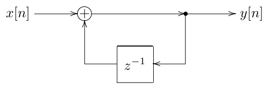
Figure 3.1: Naive integrator for T = 1.
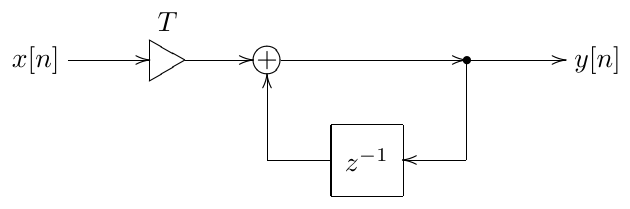
Figure 3.2: Naive integrator for arbitrary T.
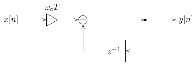
Figure 3.3: Naive integrator with embedded cutoff.
Now let’s construct the block diagram of the naive 1-pole lowpass filter. Recalling the implementation routine:
// perform one sample tick of the lowpass filter
y := y + (x-y)*omega_c;
we obtain the diagram in Fig. 3.4. The element in the feedback from the filter’s output to the leftmost summator is occurring due to the fact that we are picking up the previous value of in the routine when computing the difference .
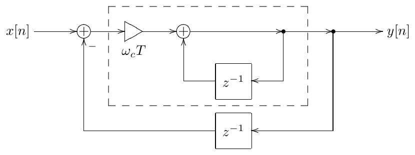
Figure 3.4: Naive 1-pole lowpass filter (the dashed line denotes the integrator).
This unit delay occurring in the discrete-time feedback is a common problem in discrete-time implementations. This problem is solvable, however it doesn’t make too much sense to solve it for the naive integrator-based models, as the increased complexity doesn’t justify the improvement in sound. We will address the problem of the zero-delay discrete-time feedback later, for now we’ll concentrate on the naive model in Fig. 3.4. This model can be simplified a bit, by combining the two elements into one (Fig. 3.5), so that the block diagram explicitly contains a single state variable (as does its pseudocode counterpart).
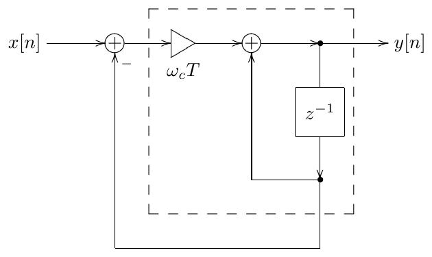
Figure 3.5: Naive 1-pole lowpass filter with just one element (the dashed line denotes the integrator).
3.5 Transfer function
Let and be respectively the input and the output signals of a unit delay:
For a complex exponential input we obtain
That is
That is, is the transfer function of the unit delay! It is common to express discrete-time transfer functions as functions of rather than functions of . The reason is that in this case the transfer functions are nonstrictly proper6 rational functions, similarly to the continuous-time case, which is pretty convenient. So, for a unit delay we could write .
Now we can obtain the transfer function of the naive integrator in Fig. 3.1. Suppose7 and , or shortly, and . Then the output of the element is . The output of the summator is then , thus
from where
and
This is the transfer function of the naive integrator (for ).
It is relatively common to express discrete-time transfer functions as rational functions of (like the one above) rather than rational functions of . However, for the purposes of the analysis it is also often convenient to have them expressed as rational functions of (particularly, for finding their poles and zeros). We can therefore multiply the numerator and the denominator of the above by , obtaining:
Since , the frequency response is obtained as . The amplitude and phase responses are and respectively.8
For we obtain
and, since , the frequency response is .
Now let’s obtain the transfer function of the naive 1-pole lowpass filter in Fig. 3.5, where, for the simplicity of notation, we assume . Assuming complex exponentials and we have and as the inputs of the first summator. Respectively the integrator’s input is . And the integrator output is the sum of and the integrator’s input. Therefore
From where
and
The transfer function for can be obtained by simply replacing by .
The respective amplitude response is plotted in Fig. 3.6. Comparing it to the amplitude response of the analog prototype we can observe serious deviation closer to the Nyquist frequency. The phase response (Fig. 3.7) has similar deviation problems.
In principle, the amplitude response deviation can be drastically reduced by correcting the filter’s cutoff setting. E.g. one could notice that the second of the amplitude responses in Fig. 3.6 is occurring a bit too far to the right, compared to the analog response (which is what we’re aiming at). Therefore we could achieve a better matching between the two responses by reducing the cutoff setting of the digital filter by a small amount. Depending on the formal definition of the response matching, one could derive an analytical expression for such cutoff correction. There are two main problems with that, though.
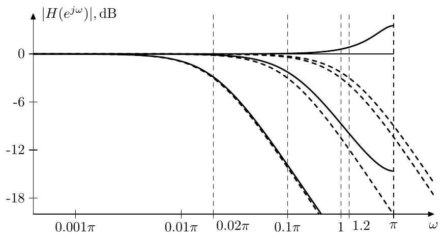
Figure 3.6: Amplitude response of a naive 1-pole lowpass filter for a number of different cutoffs. Dashed curves represent the respective analog filter responses for the same cutoffs.
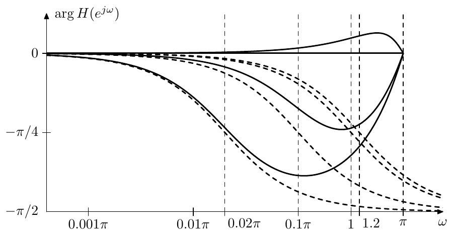
Figure 3.7: Phase response of a naive 1-pole lowpass filter for a number of different cutoffs. Dashed curves represent the respective analog filter responses for the same cutoffs.
One problem is that many other filters, e.g. a 2-pole resonating lowpass, have more parameters, e.g. not only cutoff but also the resonance, and we potentially may need to correct all of them, which results in much more involved math. This problem is not as critical though, and there are some methods utilizing this approach.
The other problem, though, is the phase response. Looking at Fig. 3.7 it seems that no matter how we try to correct the filter’s cutoff, the phase response will be always zero at Nyquist, whereas we would desire something close to . The effects of the deviation of the filter’s phase response are mostly quite subtle. Therefore it’s somewhat difficult to judge how critical the phase devations might be.9 However there’s one absolutely objective and major issue associated with the phase deviations. Attempting to mix outputs of two filters with some deviations in either or both of the amplitude and phase responses may easily lead to unexpected and undesired results. For that reason in this book we will concentrate on a different method which is much more robust in this respect.
Poles and zeros
Discrete-time block diagrams are differing from continuous-time block diagrams only by having elements instead of integrators. Recalling that the transfer function of an integrator is , we conclude that from the formal point of view the difference is purely notational.
Now, the transfer functions of continuous-time block diagrams are non- strictly proper rational functions of . Respectively, the transfer functions of discrete-time block diagrams are nonstrictly proper rational functions of .
Thus, discrete-time transfer functions will have poles and zeros in a way similar to continuous-time transfer functions. Similarly to continuous-time transfer functions, the poles will define the stability of a linear time-invariant filter. Consider that and recall the stability criterion (where , where are the poles). Apparently, . We might there- fore intuitively expect the discrete-time stability criterion to be where are the discrete-time poles. This is indeed the case, a linear time-invariant difference system10 is stable if and only if all its poles are located inside the unit circle. We will give more detail about the mechanisms behind this in the discussion of the discrete-time transient response in Sections 3.12 and 7.13.
3.6 Trapezoidal integration
Instead of naive integration, we could attempt using the trapezoidal integration method ():
// perform one sample tick of the integrator
integrator_output := integrator_output +
    (integrator_input + previous_integrator_input)/2;
previous_integrator_input := integrator_input;
Notice that now we need two state variables per integrator: integrator_output and previous_integrator_input. The block diagram of a trapezoidal integrator is shown in Fig. 3.8. We’ll refer to this integrator as a direct form I trapezoidal integrator. The reason for this term will be explained later.
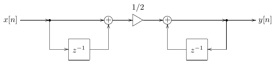
Figure 3.8: Direct form I trapezoidal integrator (T = 1).
We could also construct a trapezoidal integrator implementation with only a single state variable. Consider the expression for the trapezoidal integrator’s output:
Suppose and , corresponding to a zero initial state (recall that both and are technically stored in the elements). Then
where
Now notice that is the output of a naive integrator, whose input signal is . At the same time is the average of the previous and the current output values of the naive integrator. This can be implemented by the structure in Fig. 3.9. Similar considerations apply for nonzero initial state. We’ll refer to the integrator in Fig. 3.9 as a direct form II or canonical trapezoidal integrator. The reason for this term will be explained later.
We can develop yet another form of the bilinear integrator with a single state variable. Let’s rewrite (3.2) as
and let
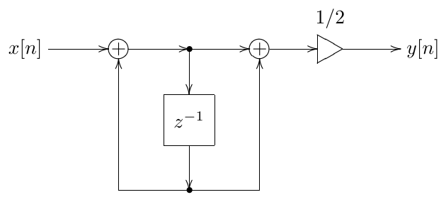
Figure 3.9: Direct form II (canonical) trapezoidal integrator (T = 1).
Notice that
and
Expressing (3.3a) and (3.3b) in a graphical form, we obtain the structure in Fig. 3.10. We’ll refer to the integrator in Fig. 3.10 as a transposed direct form II or transposed canonical trapezoidal integrator. The reason for this term will be explained later.
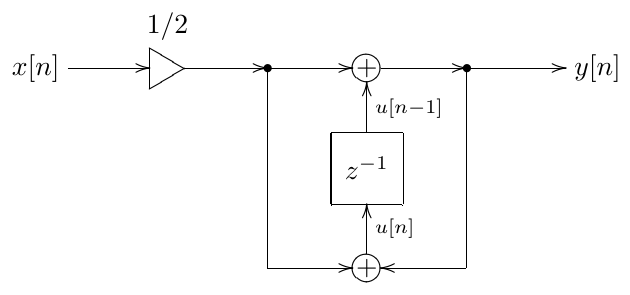
Figure 3.10: Transposed direct form II (transposed canonical) trapezoidal integrator (T = 1).
The positioning of the 1/2 gain prior to the integrator in Fig. 3.10 is quite convenient, because we can combine the 1/2 gain with the cutoff gain into a single gain element. In case of an arbitrary sampling period we could also include the factor into the same gain element, thus obtaining the structure in Fig. 3.11. A similar trick can be performed for the other two integrators, if we move the 1/2 gain element to the input of the respective integrator. Since the integrator is a linear time-invariant system, this doesn’t affect the integrator’s behavior in a slightest way.
Typically one would prefer the direct form II integrators to the direct form I integrator, because the former have only one state variable. In this book we will mostly use the transposed direct form II integrator, because this is resulting in slightly simpler zero-delay feedback equations and also offers a nice possibility for the internal saturation in the integrator.
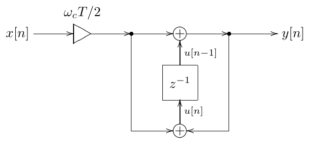
Figure 3.11: Transposed direct form II (transposed canonical) trapezoidal integrator with “embedded” cutoff gain.
The transfer functions of all three integrators are identical. Let’s obtain e.g. the transfer function of the transposed canonical integrator (in Fig. 3.10). Assuming signals of the exponential form , we can drop the index , under- standing it implicity, while the index will be replaced by the multiplication by . Then (3.3) turn into
Substituting the second equation into the first one we have
and the transfer function of the trapezoidal integrator is thus
For an arbitrary one has to multiply the result by , to take the respective gain element into account:
If also the cutoff gain is included, we obtain
One can obtain the same results for the other two integrators.
What is so special about this transfer function, that makes the trapezoidal integrator so superior to the naive one, is to be discussed next.
3.7 Bilinear transform
Suppose we take an arbitrary continuous-time block diagram, like the familiar lowpass filter in Fig. 2.2 and replace all continuous-time integrators by discrete- time trapezoidal integrators. On the transfer function level, this will correspond to replacing all with . That is, technically we perform a substitution
in the transfer function expression.
It would be more convenient to write this substitution explicitly as
The substitution (3.4) is referred to as the bilinear transform, or shortly BLT. For that reason we can also refer to trapezoidal integrators as BLT integrators. Let’s figure out, how does the bilinear transform affect the frequency response of the filter, that is, what is the relationship between the original continuous- time frequency response prior to the substitution and the resulting discrete-time frequency response after the substitution.
Let be the original continuous-time transfer function. Then the re- spective discrete-time transfer function is
Respectively, the discrete-time frequency response is
Notice that in the last expression is evaluated on the imaginary axis!!! That is, the bilinear transform maps the imaginary axis in the -plane to the unit circle in the -plane! Now, is the analog frequency response evaluated at . That is, the digital frequency response at is equal to the analog frequency response at . This means that the analog fre- quency response in the range is mapped into the digital frequency range (), that is from zero to Nyquist!11 Denoting the analog frequency as and the digital frequency as we can express the argument mapping of the frequency response function as
or, in a more symmetrical way
Notice that for frequencies much smaller that Nyquist frequency we have and respectively .
This is what is so unique about the bilinear transform. It simply warps the frequency range into the zero-to-Nyquist range, but otherwise doesn’t change the frequency response at all! Considering in comparison a naive inte- grator, we would have obtained:
which means that the digital frequency response is equal to the analog transfer function evaluated on a circle of radius 1 centered at . This hardly defines a clear relationship between the two frequency responses.
So, by simply replacing the analog integrators with digital trapezoidal in- tegrators, we obtain a digital filter whose frequency response is essentially the same as the one of the analog prototype, except for the frequency warping. Particularly, the relationship between the amplitude and phase responses of the filter is fully preserved, which is particularly highly important if the filter is to be used as a building block in a larger filter. Very close to perfect!
Furthermore, the bilinear transform maps the left complex semiplane in the -domain into the inner region of the unit circle in the -domain. Indeed, let’s obtain the inverse bilinear transform formula. From (3.4) we have
from where
and
The equation (3.9) defines the inverse bilinear transform. Now, if , then, obviously
and . Thus, the left complex semiplane in the -plane is mapped to the inner region of the unit circle in the -plane. In the same way one can show that the right complex semiplane is mapped to the outer region of the unit circle. And the imaginary axis is mapped to the unit circle itself. Comparing the stability criterion of analog filters (the poles must be in the left complex semiplane) to the one of digital filters (the poles must be inside the unit circle), we conclude that the bilinear transform exactly preserves the stability of the filters!
In comparison, for a naive integrator replacement we would have the follow- ing. Inverting the (3.8) substitution we obtain
and
Assuming and considering that in this case
we conclude that the left semiplane is mapped into a circle of radius 0.5 cen- tered at . So the naive integrator overpreserves the stability, which is not nice, since we would rather have digital filters behaving as closely to their analog prototypes as possible. Considering that this comes in a package with a poor frequency response transformation, we should rather stick with trapezoidal integrators.
So, let’s replace e.g. the integrator in the familiar lowpass filter structure in Fig. 2.2 with a trapezoidal integrator. Performing the integrator replacement, we obtain the structure in Fig. 3.12.12 We will refer to the trapezoidal integrator replacement method as the topology-preserving transform (TPT) method. This term will be explained and properly introduced later. For now, before we simply attempt to implement the structure in Fig. 3.12 in code, we should become aware of a few further issues.
3.8 Cutoff prewarping
Suppose we are using the lowpass filter structure in Fig. 3.12 and we wish to have its cutoff at . If we however simply put this parameter into the respective integrator gain element , the frequency response itself and, specifically, its value at the cutoff will be different from the expected one. Fig. 3.13 illustrates. The dB level is specifically highlighted in Fig. 3.13, since this is the amplitude response value of the 1-pole lowpass filter at the cutoff, thereby aiding the visual identification of the cutoff point on the response curves.13
Apparently, the difference between analog and digital response is occuring due to the warping of the frequency axis (3.6). We would like to estimate the frequency error introduced by the warping. To simplify the further discussion let’s rewrite (3.6) as a mapping function :
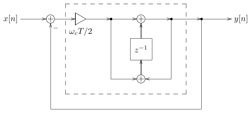
Figure 3.12: 1-pole TPT lowpass filter (the dashed line denotes the trapezoidal integrator).
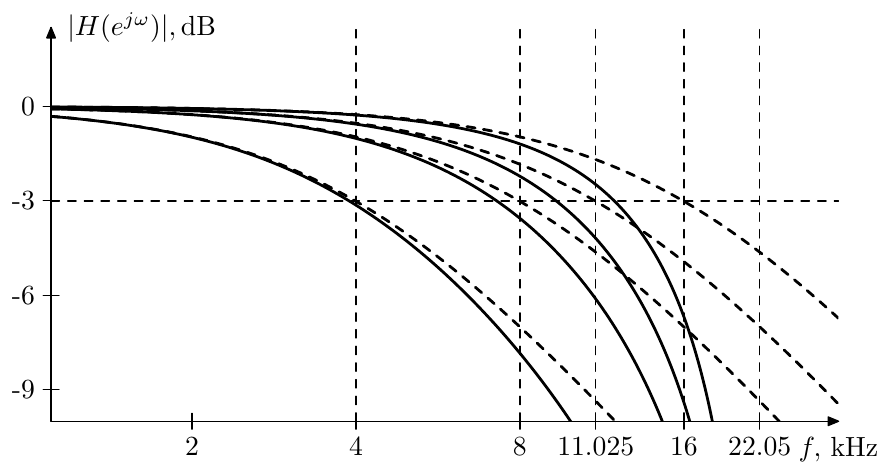
Figure 3.13: Amplitude response of an unprewarped bilinear-transformed 1-pole lowpass filter for a number of different cutoffs. Dashed curves represent the respective analog filter responses for the same cutoffs. Sampling rate 44.1kHz.
Now, given some desired analog response, we could take some point on this response and ask ourselves, where is the same point located on the digital response. According to (3.10), it is located at (where is the function inverse of ). Thus the ratio of the actual and desired frequencies is , or, in the octave scale:
The solid curve in Fig. 3.14 illustrates (note that Fig. 3.14 labels the axis in semitones).
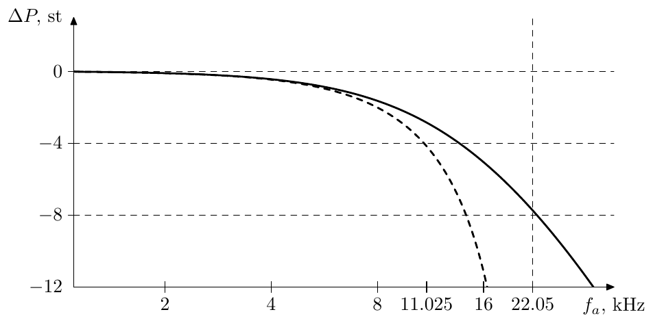
Figure 3.14: Bilinear transform’s detuning of analog frequencies plotted against analog frequency (solid curve) or digital frequency (dashed curve). Sampling rate 44.1kHz.
We could also express the detuning of analog frequencies in terms of the corresponding digital frequency. Given the digital frequency response, we take some point and ask ourselves, where is the same point located on the analog response. According to (3.10), it is located at and thus the frequency ratio is , respectively
The dashed curve in Fig. 3.14 illustrates. Note that we are not talking about how much the specified digital frequency will be detuned (because digital frequencies are not getting detuned, they are already where they are), it’s still about how much the corresponding analog frequency will be detuned.
Thus, given an analog filter with a frequency response , its digital counterpart will have its frequencies detuned as shown in Fig. 3.14. Particularly, the cutoff point, instead of being at the specified frequency , will be at
In principle, one could argue that the frequency response change in Fig. 3.13 is not that drastic and could be tolerated, especially since the deviation occurs mostly in the high frequency range, which is not the most audible part of the frequency spectrum. This might have been the case with the 1-pole lowpass filter, however for other filters with more complicated amplitude responses it won’t be as acceptable. Fig. 3.15 illustrates the frequency error for a 2-pole resonating lowpass filter. The resonance peaks (which occur close to the filter’s cutoff) are very audible and so would be their detuning, which according to Fig. 3.14 is in the range of semitones. Particularly, at 16kHz the dashed curve in Fig. 3.14 shows a detuning of ca. 1 octave, meaning that we would have a resonance at this point when it should have been occurring at ca. 32kHz.
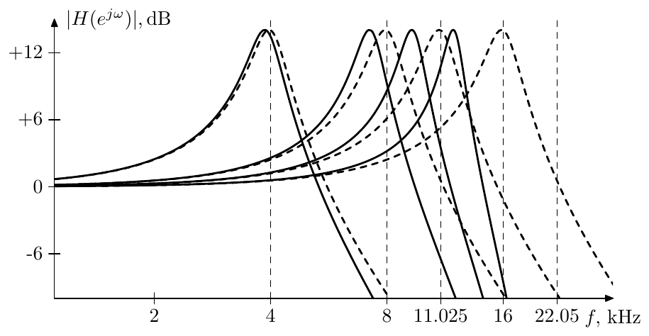
Figure 3.15: Amplitude response of an unprewarped bilinear-transformed resonating 2-pole lowpass filter for a number of different cutoffs. Dashed curves represent the respective analog filter responses for the same cutoffs. Sampling rate 44.1kHz.
Prewarping at cutoff
As a general rule (to which there are exceptions), we would like the cutoff point of the filter to be positioned exactly at the specified cutoff frequency . In this regard we could notice that if we used a different cutoff value
then (3.11) would give
and the cutoff point would be exactly where we wanted it to be. Fig. 3.16 illus- trates. The cutoff correction (3.12) is a standard technique used in combination with the bilinear transform. It is referred to as cutoff prewarping.
Technically, cutoff prewarping means that we use instead of in the gains of the filter’s integrators. However, the integrator gains are not exactly but rather . From (3.12) and (3.10) we have
Thus, we can directly apply (3.13) to compute the prewarped gains . Note that (3.13) is essentially identical to (3.7).
The cutoff prewarping redistributes the frequency error shown in Fig. 3.14. In the absence of prewarping the error was zero at and monotonically growing as increases. With the cutoff prewarping the error is zero at instead and grows further away from this point.
Indeed, let be unit-cutoff analog response of the filter in question. And let’s pick up an analog frequency and find the respective detuning. The correct frequency response at is
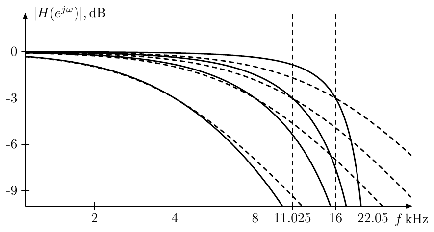
Figure 3.16: Amplitude response of a prewarped bilinear-transformed 1-pole lowpass filter for a number of different cutoffs. Dashed curves represent the respective analog filter responses for the same cutoffs. Sampling rate 44.1kHz.
On the other hand, given the prewarped cutoff , the digital frequency response at some frequency is
We want to find such that the arguments of in (3.14a) and (3.14b) are identical:
From where
The solid curves in Fig. 3.17 illustrate the respective detuning (in semi- tones) of analog frequencies.
Alternatively from (3.15) we could express as a function of :
thus expressing the analog frequency detuning as a function of . The dashed curves in Fig. 3.17 illustrate.
Apparently, the maximum error to the left of is attained at . Letting and, equivalently, we have and (3.15) turns into
or
and thus the detuning at is
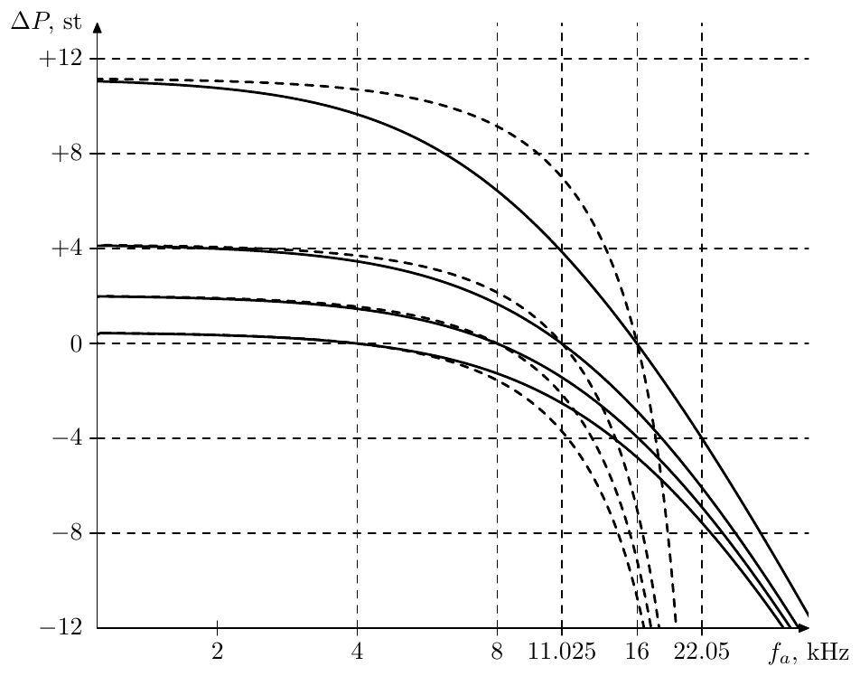
Figure 3.17: Prewarped bilinear transform’s detuning of analog frequencies plotted against analog frequency (solid curves) or digital frequency (dashed curves). Different curves correspond to prewarping at different cutoff frequencies. Sampling rate 44.1kHz.
Other prewarping points
We have just developed the prewarping technique from the condition that the cutoff point must be preserved by the mapping (3.6). However instead we could have required any other point to be preserved.
Given the cutoff , the analog response at is
On the other hand, given the prewarped cutoff (we want to prewarp at a different point now, therefore we don’t know yet, what is the relationship between and ) the digital frequency response at is
We want to find such that the arguments of in (3.17a) and (3.17b) are identical:
and
Equation (3.18) is the generalized prewarping formula, where is the frequency response point of zero detuning. We will refer to as the prewarping point.
According to (3.18) prewarping at simply means that the cutoff should be multiplied by . At this multiplication reduces to (3.12).
In order to find the detuning at other frequencies, notice that equations (3.14) turn into
from where, equating the arguments of :
we have
Equation (3.19) is identical to (3.15) except that it has in place of . Thus we could reuse the results of the previous analysis of the analog frequency detuning. In particular Fig. 3.17 fully applies, different curves corresponding to different prewarping points. At the same time, (3.16) simply turns to
Bounded cutoff prewarping
Even though cutoff prewarping is an absolutely standard technique and is often used without any second thought, the need for a different choice of the prewarping point is actually not as exotic as it might seem. Consider e.g. the amplitude response of a 1-pole highpass filter prewarped by (3.12), shown in Fig. 3.18. One can notice a huge discrepancy between analog and digital amplitude responses occurring well into the audible frequency range . The error is getting particularly bad at cutoffs above 16kHz. In comparison, the responses of unprewarped filters in Fig. 3.19 even look kind of better, especially if only the audible frequency range is considered. This would be even more so, if higher sampling rates were involved, where the audible range error in Fig. 3.19 would become smaller, while the same error in Fig. 3.18 can still get as large, given a sufficiently high cutoff value.
Apparently, the large error within the audible range in Fig. 3.18 is due to the detuning error illustrated in Fig. 3.17. This error wasn’t as obvious in the case of the 1-pole lowpass filter, since this filter’s amplitude response is almost constant to the left of the cutoff point. On the other hand, highpass filter’s amplitude response is changing noticeably in the same area, which makes the detuning error is made much more promiment.
Does this suggest that we shouldn’t use cutoff prewarping with highpass filters? In principle this is engineer’s decision. However consider the unprewarped resonating 2-pole highpass filter’s amplitude response in Fig. 3.20. As with the responating lowpass, the resonance peak detuning is quite prominent here. Also the difference in the response value is magnified around the resonance point. All in all, we’d rather prewarp the cutoff (Fig. 3.21) and tolerate the detuning to the left of .
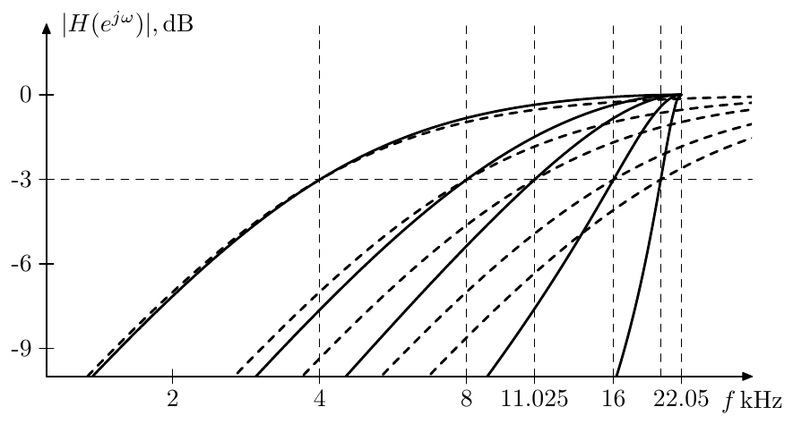 Figure 3.18: Amplitude response of a prewarped bilinear-transformed 1-pole highpass filter for a number of different cutoffs. Dashed curves represent the respective analog filter responses for the same cutoffs. Sampling rate 44.1kHz.
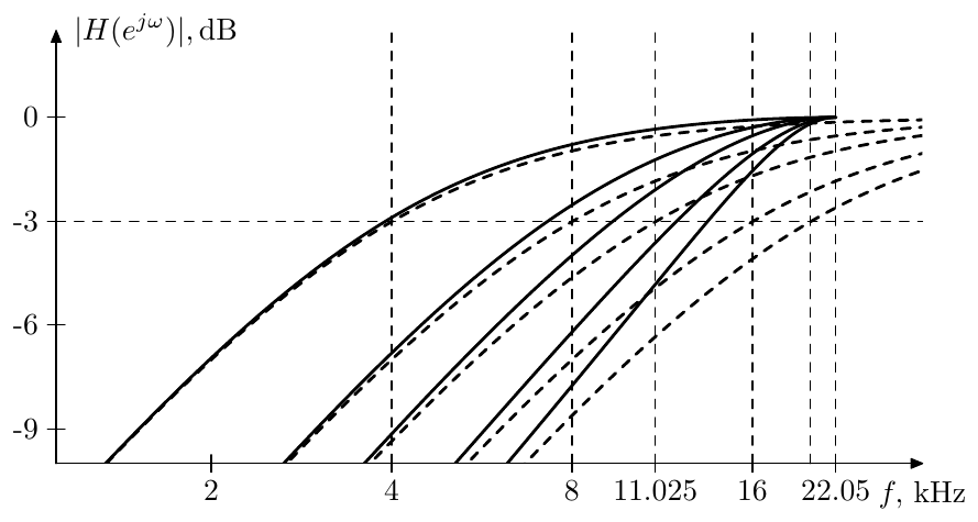 Figure 3.19: Amplitude response of an unprewarped bilinear-transformed 1-pole highpass filter for a number of different cutoffs. Dashed curves represent the respective analog filter responses for the same cutoffs. Sampling rate 44.1kHz.
However notice, that as the cutoff peak is getting out of the audible range, we stop caring, where exactly it is positioned, since it can’t be heard anyway. So, why should we then tolerage the error in the audible range which continues to increase even faster? Instead, at this moment we could fix the prewarping point to the upper boundary of the audible range:
or simply
where is some point around 16kHz. At least then the detuning in the audible range won’t grow any further than it is at (Fig. 3.22). The picture gets even better at higher sampling rates (Fig. 3.23).
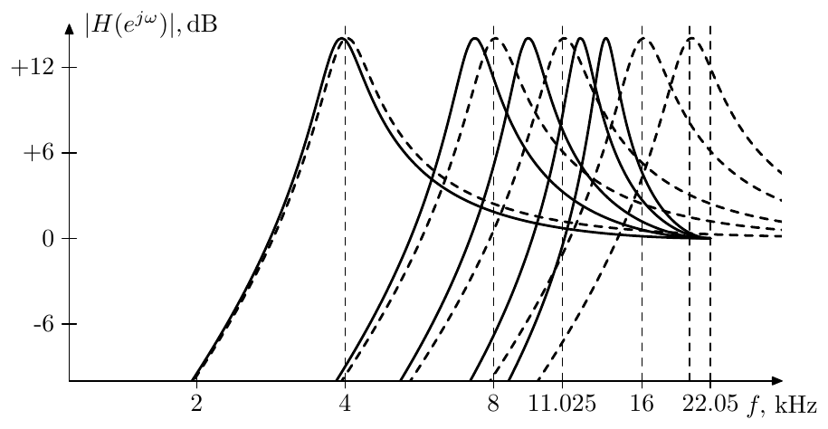 Figure 3.20: Amplitude response of an unprewarped bilinear-transformed resonating 2-pole highpass filter for a number of different cutoffs. Dashed curves represent the respective analog filter responses for the same cutoffs. Sampling rate 44.1kHz.
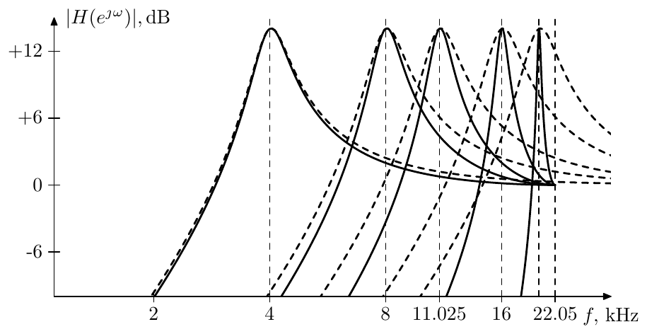 Figure 3.21: Amplitude response of a prewarped bilinear-transformed resonating 2-pole highpass filter for a number of different cutoffs. Dashed curves represent the respective analog filter responses for the same cutoffs. Sampling rate 44.1kHz.
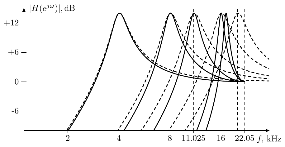 Figure 3.22: Effect of cutoff prewarping bounded at 16kHz. Sampling rate 44.1kHz.
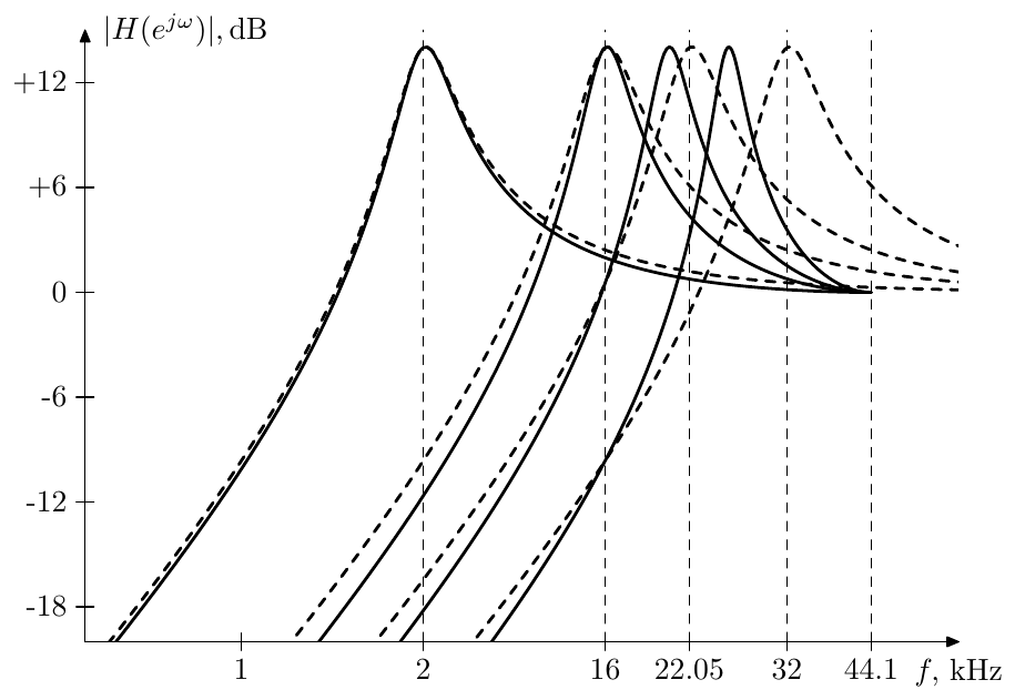 Figure 3.23: Effect of cutoff prewarping bounded at 16kHz. Sampling rate 88.1kHz.
Substituting (3.21) into (3.18) we obtain
The mapping defined by (3.22) is shown in Fig. 3.24. Note that thereby we become able to specify the cutoffs beyond Nyquist, and actually to specify arbitrarily large cutoffs, since the new mapping curve is crossing the former vertical asymptote at .
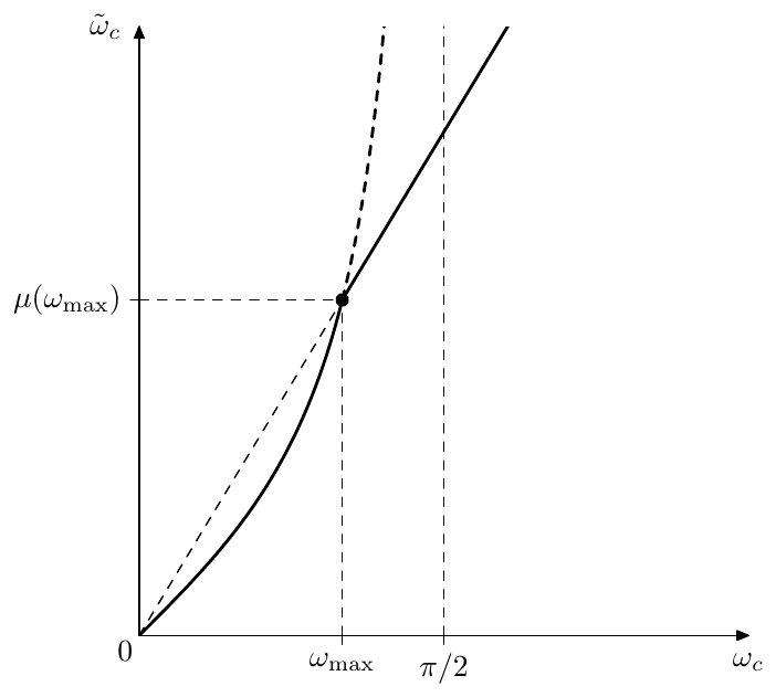 Figure 3.24: Bounded cutoff prewarping. The thick dashed line shows the unbounded prewarping continuation. The thin oblique dashed line is the continuation of the straight part of the prewarping curve. The black dot marks the breakpoint of the prewarping curve.
The breakpoint at in Fig. 3.24 can be somewhat unexpected. In order to understand the mechanism behind its appearance suppose is varying with time. Using (3.18) we compute the time derivative of :
As becomes larger than the first term suddenly disappears and there is a jump in . In other words, the variation of the prewarping point makes its own contribution to . As soon as the variation stops, the respective contribution abruptly disappears.
The frequency detunings occurring in case of (3.22) can be found directly from Fig. 3.17, keeping in mind that (3.22) is simply another expression of (3.21).
Continuous-speed prewarping
The breakpoint occurring in Fig. 3.24 might be undesirable if the cutoff is being modulated, since there can be a sudden change of the perceived modulation speed as the cutoff traverses through the prewarping breakpoint. For that reason it might be desirable to smooth the breakpoint in one way or the other. The simplest approach would be to continue the curve as a tangent line after the breakpoint:
where
is the derivative of . Note, however, that this will no longer keep as the prewarping point and the situation would be something in between (3.12) and (3.22).
At from (3.23) we have
Comparing the right-hand side of (3.24) to (3.18) we obtain the equation for the effective prewarping point at infinity:
In principle can be found from (3.25), however we are not so much interested in how far off will be the prewarping point, as in the estimation of the associated increase in detuning. By (3.20)
which for kHz at 44.1kHz sampling rate gives ca. 2.5 octaves, while at 88.2kHz sampling rate it gives only about 0.5 octave. In comparison, at (and respectively ) we would have a smaller value
which for kHz at 44.1kHz sampling rate gives ca. 1 octave, while at 88.2kHz sampling rate it gives only about 2 semitones.
We have therefore found the effect of (3.23) on the detuning occurring at for . It would also be nice to estimate the same effect at . By (3.19)
which by (3.25) becomes
Letting we have
and the detuning itself is the logarithm of the ratio
For kHz at 44.1kHz sampling rate this gives ca. octaves, while at 88.1kHz it gives ca. semitones.
Since (as illustrated by Fig. 3.17) the detuning is a monotonic function of , at we are having the audible range detuning error in the range of ca. octaves at 44.1kHz sampling rate and in the range of ca. semitones at 88.2kHz sampling rate. Therefore it is more or less balanced out, although being a bit larger at higher frequencies.
Apparently, more elaborate ways of smoothing the breakpoint in Fig. 3.24 may be designed, but we won’t cover them here as the options are almost infinite.
Prewarping of systems of filters
According to (3.18), prewarping is nothing more than a multiplication of the cutoff gains of the integrators by , where is the prewarping point.
Suppose we are having a system consisting of several filters connected together. When prewarping filters in such system, it would be a good idea to choose a common prewarping point for all filters. In this case we multiply their cutoffs by one and the same coefficient. Thereby their amplitude and phase responses are shifted by one and the same amount (in the logarithmic frequency axis), and they all retain the frequency response relationships which existed between them prior to prewarping. Effectively this is the same as changing the “common cutoff” of the filter system, and the frequency response of the entire system is simply shifted horizontally by the same amount, fully retaining its shape.
On the other hand by prewarping them independently we shift the frequency response of each filter differently from the others and the amplitude and phase relationships between those are thereby destroyed. Therefore the amplitude and phase response shapes of the entire system of filters are not preserved.
As an illustration consider a parallel connection of a 1-pole lowpass and a 1-pole highpass filter, the lowpass cutoff being , the highpass cutoff being where is the formal cutoff of the system:
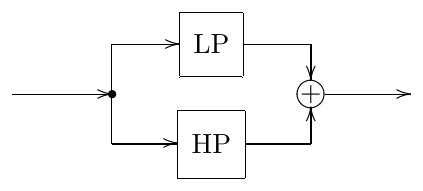
The transfer function of such system (written in the unit-cutoff form) is
The result of prewarping the lowpass and the highpass separately at their respective cutoffs and is shown in Fig. 3.25. Actually for the kHz and kHz the highpass cutoff needed to be clipped prior to prewaring, since it is equal or exceeds Nyquist and cannot be directly prewarped by (3.12). Compare to Fig. 3.26 where the prewarping of both filters has been done at the common point .
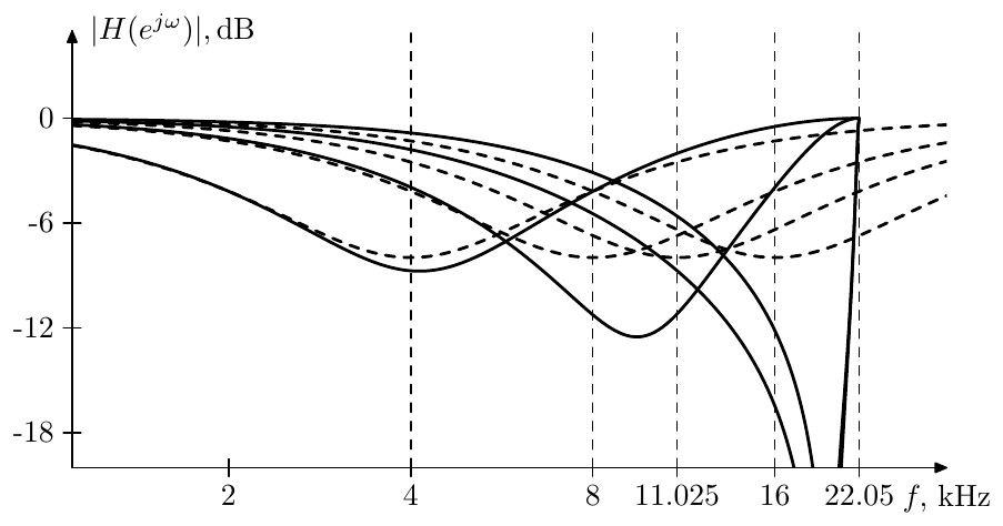 Figure 3.25: Separate prewarping of system components (for a number of different cutoffs). Dashed curves represent the respective analog filter responses for the same cutoffs. Sampling rate 44.1kHz.
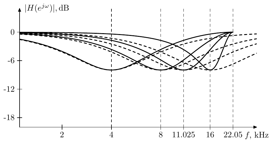 Figure 3.26: Common-point prewarping of system components (for a number of different cutoffs). Dashed curves represent the respective analog filter responses for the same cutoffs. Sampling rate 44.1kHz.
Other prewarping techniques
With 1-pole lowpass and highpass filters the only available control parameter is the filter cutoff. Thus the only option which we had for compensating the bilinear transform’s frequency detuning was correcting the cutoff value. Other filters may have more parameters available. Usually their parameters (e.g. resonance) will have a strong “vertical” effect on the amplitude response and thus are not very suitable for compensating the frequency detuning. However in some cases there will be further options of horizonally altering the filter’s amplitude (and phase) responses without causing noticeable changes in the vertical direction. In such cases we will have further options for more detailed compensation of the frequency detuning.
Note, however, that these compensations, being not expressible as cutoff multiplication, may destroy the frequency response of a system of filters, unless there is some other way to make them have identical effect on all of the filters in the system. We will discuss some examples of this later in the book.
3.9 Zero-delay feedback
There is a further problem with the trapezoidal integrator replacement in the TPT method. Replacing the integrators with trapezoidal ones introduces delayless feedback loops (that is, feedback loops not containing any delay elements) into the structure. E.g. consider the structure in Fig. 3.12. Carefully examining this structure, we find that it has a feedback loop which doesn’t contain any unit delay elements. This loop goes from the leftmost summator through the gain, through the upper path of the integrator to the filter’s output and back through the large feedback path to the leftmost summator.
Why is this delayless loop a problem? Let’s consider for example the naive lowpass filter structure in Fig. 3.5. Suppose we don’t have the respective program code representation and wish to obtain it from the block diagram. We could do it in the following way. Consider Fig. 3.27, which is the same as Fig. 3.5, except that it labels all signal points. At the beginning of the computation of a new sample the signals and are already known. is the current input sample and is taken from the internal state memory of the element. Therefore we can compute . Then we can compute and finally . The value of is then stored into the internal memory of the element (for the next sample computation) and is also sent to the output as the new value. Easy, right?
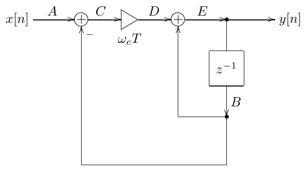 Figure 3.27: Naive 1-pole lowpass filter and the respective signal computation order.
Now the same approach doesn’t work for the structure in Fig. 3.12. Because there is a delayless loop, we can’t find a starting point for the computation within that loop.
The classical way of solving this problem is exactly the same as what we had in the naive approach: introduce a into the delayless feedback, turning it into a feedback containing a unit delay (Fig. 3.28). Now there are no delayless feedback paths and we can arrange the computation order in a way similar to Fig. 3.27. This however destroys the resulting frequency response, because the transfer function is now different. In fact the obtained result is not significantly better (if better at all) than the one from the naive approach. There are some serious artifacts in the frequency response closer to the Nyquist frequency, if the filter cutoff is sufficiently high.
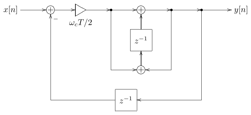 Figure 3.28: Digital 1-pole lowpass filter with a trapezoidal integrator and an extra delay in the feedback.
Therefore we shouldn’t introduce any modifications into the structure and solve the zero-delay feedback problem instead. The term “zero-delay feedback” originates from the fact that we avoid introducing a one-sample delay into the feedback (like in Fig. 3.28) and instead keep the feedback delay equal to zero.
So, let’s solve the zero-delay feedback problem for the structure in Fig. 3.12. Notice that this structure simply consists of a negative feedback loop around a trapezoidal integrator, where the trapezoidal integrator structure is exactly the one from Fig. 3.11. We will now introduce the concept of the instantaneous response of this integrator structure.
So, consider the integrator structure in Fig. 3.11. Since there are no delayless loops in the integrator, it’s not difficult to obtain the following expression for :
Notice that, at the time arrives at the integrator’s input, all values in the right-hand side of (3.26) are known (no unknown variables). Introducing notation
we have
or, dropping the discrete time argument notation for simplicity,
That is, at any given time moment , the output of the integrator is a linear function of its input , where the values of the parameters of this linear function are known. The parameter doesn’t depend on the internal state of the integrator, while the parameter does depend on the internal state of the integrator. We will refer to the linear function as the instantaneous response of the integrator at the respective implied time moment . The coefficient can be referred to as the instantaneous response gain or simply instantaneous gain. The term can be referred to as the instantaneous response offset or simply instantaneous offset.
Let’s now redraw the filter structure in Fig. 3.12 as in Fig. 3.29. We have changed the notation from to in the expression to avoid the confusion with the input signal of the entire filter.
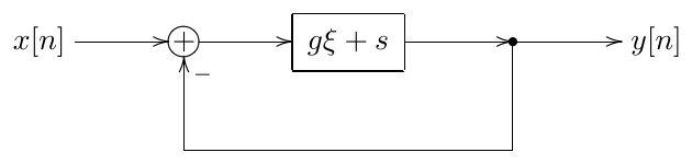
Figure 3.29: 1-pole TPT lowpass filter with the integrator in the instantaneous response form.
Now we can easily write and solve the zero-delay feedback equation. Indeed, suppose we already know the filter output . Then the output signal of the feedback summator is and the output of the integrator is respectively . Thus
or, dropping the time argument notation for simplicity,
The equation (3.27) is the zero-delay feedback equation for the filter in Fig. 3.29 (or, for that matter, in Fig. 3.12). Solving this equation, we obtain
and respectively
Having found (that is, having predicted the output ), we can then proceed with computing the other signals in the structure in Fig. 3.12, beginning with the output of the leftmost summator.14
It’s worth mentioning that (3.28) can be used to obtain the instantaneous response of the entire filter from Fig. 3.12. Indeed, rewriting (3.28) as
and introducing notations
we have
So, the instantaneous response of the entire lowpass filter in Fig. 3.12 is again a linear function of the input. We could use the expression (3.29) e.g. to solve the zero-delay feedback problem for some larger feedback loop containing a 1-pole lowpass filter.
3.10 Implementations
1-pole lowpass
We are now going to convert the structure in Fig. 3.12 into a piece of code. Let’s introduce helper variables into Fig. 3.12 as shown in Fig. 3.30, where we have used the already known to us fact that, given the integrator’s instantaneous response , the value of equals the output of the element.
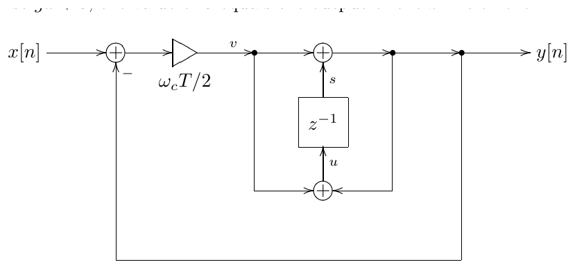
Figure 3.30: 1-pole TPT lowpass filter with helper variables.
We already know from (3.29). Since , we have
Now (3.30) gives a direct expression for in terms of known signals, not using . In order to avoid unnecessary computations, we can simply reobtain using the obvious from Fig. 3.30 fact that is just a sum of and :
We also need the input (which we need to store in the ’s memory) which is also obtained from Fig. 3.30 in an obvious way:
The equations (3.30), (3.31) and (3.32) can be directly expressed in program code:
// perform one sample tick of the lowpass filter
// G = g/(1+g)
// the variable 's' contains the state of z^-1 block
v := (x-s)*G;
y := v + s;
s := y + v;
or instead expressed in a block diagram form (Fig. 3.31). Notice that the block diagram doesn’t contain any delayless loops anymore.
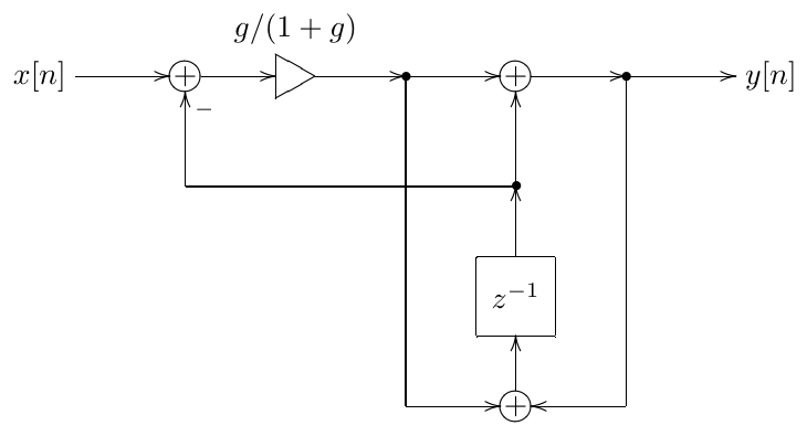
Figure 3.31: 1-pole TPT lowpass filter with resolved zero-delay feedback.
1-pole multimode
The highpass signal can be obtained from the structure in Fig. 3.31 in a trivial manner, since , thereby turning Fig. 3.31 into a multimode 1-pole.
1-pole highpass
If we need only the highpass signal, we could do it in a smaller number of operations than in the multimode 1-pole. By noticing that
and that
we can implement the highpass filter as follows:
// perform one sample tick of the highpass filter
// Ghp = 1/(1+g)
// the variable 's' contains the state of z^-1 block
xs := x - s;
y := xs*Ghp;
s := s + y*2g;
however this way we have traded an addition/subtraction pair for one multiplication, plus instead of one cutoff-dependent parameter we need to store and access Ghp and 2g. Therefore this is not necessarily a performance improvement.
1-pole allpass
The allpass signal can be obtained from the multimode 1-pole in a trivial manner, recalling that . However, if we need only the allpass signal, we could save a couple of operations. Noticing that
and that is the new state of the block, we obtain
// perform one sample tick of the allpass filter
// 2Glp=2g/(1+g)
// the variable 's' contains the state of z^-1 block
xs := x - s;
s := s + xs*2Glp;
y := s - xs;
3.11 Direct forms
Consider again the equation (3.5), which describes the application of the bilinear transform to convert an analog transfer function to a digital one. There is a classical method of digital filter design which is based directly on this transformation, without using any integrator replacement techniques. In the author’s experience, for music DSP needs this method typically has a largely inferior quality, compared to the TPT. Nevertheless we will describe it here for completeness and for a couple of other reasons. Firstly, it would be nice to try to analyse and understand the reasons for the problems of this method. Secondly, this method could be useful once in a while. Particularly, its deficiencies mostly disappear in the time-invariant (unmodulated or sufficiently slowly modulated) case.
Having obtained a digital transfer function from (3.5), we could observe, that, since the original analog transfer function was a rational function of , the resulting digital transfer function will necessarily be a rational function of . E.g. using the familiar 1-pole lowpass transfer function
we obtain
Now, there are standard discrete-time structures allowing an implementation of any given nonstrictly proper rational transfer function. It is easier to use these structures, if the transfer function is expressed as a rational function of rather than the one of . In our particular example, we can multiply the numerator and the denominator by , obtaining
The further requirement is to have the constant term in the denominator equal to 1, which can be achieved by dividing everything by :
Now suppose we have an arbitrary rational nonstrictly proper transfer function of , expressed via and having the constant term in the denominator equal to 1:
This transfer function can be implemented by the structure in Fig. 3.32 or by the structure in Fig. 3.33. One can verify (by computing the transfer functions of the respective structures) that they indeed implement the transfer function (3.34). There are also transposed versions of these structures, which the readers should be able to construct on their own.
Let’s use the direct form II to implement (3.33). Apparently, we have
and the direct form implementation itself is the one in Fig. 3.34 (we have merged the and coefficients into a single gain element).
In the time-invariant (unmodulated) case the performance of the direct form filter in Fig. 3.34 should be identical to the TPT filter in Fig. 3.12, since both implement the same bilinear-transformed analog transfer function (2.5). When the cutoff is modulated, however, the performance will be different.
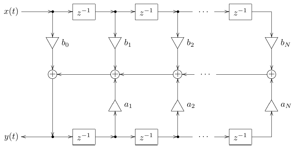
Figure 3.32: Direct form I (DF1).
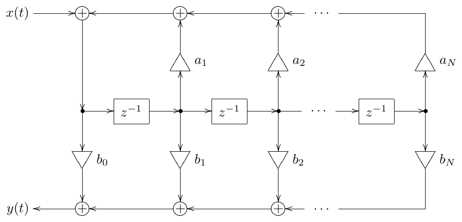
Figure 3.33: Direct form II (DF2), a.k.a. canonical form.
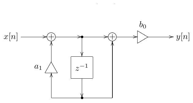
Figure 3.34: Direct form II 1-pole lowpass filter.
We have already discussed in Sections 2.7 and 2.16 that different topologies may have different time-varying behavior even if they share the same transfer function. Apparently, the difference in behavior between Fig. 3.34 and Fig. 3.12 is another example of that. Comparing the implementations in Figs. 3.34 and 3.12, we notice that the structure in Fig. 3.34 contains a gain element at the output, the value of this gain being approximately proportional to the cutoff (at low cutoffs). This will particularly produce unsmoothed jumps in the output in response to jumps in the cutoff value. In the structure in Fig. 3.12, on the other hand, the cutoff jumps will be smoothed by the integrator. Thus, the difference between the two structures is similar to the just discussed effect of the cutoff gain placement with the integrator.
We should conclude that, other things being equal, the structure in Fig. 3.34 is inferior to the one in Fig. 3.12 (or Fig. 3.31). In this respect consider that Fig. 3.12 is trying to explicitly emulate the analog integration behavior, preserving the topology of the original analog structure, while Fig. 3.34 is concerned solely with implementing a correct transfer function. Since Fig. 3.34 implements a classical approach to the bilinear transform application for digital filter design (which ignores the filter topology) we’ll refer to the trapezoidal integration replacement technique as the topology-preserving bilinear transform (or, shortly, TPBLT). Or, even shorter, we can refer to this technique as simply the topology-preserving transform (TPT), implicitly assuming that the bilinear transform is being used.15
In principle, sometimes there are possibilities to “manually fix” the structures such as in Fig. 3.34. E.g. the time-varying performance of the latter is drastically improved by moving the gain to the input. The problem however is that this kind of fixing quickly gets more complicated (if being possible at all) with larger filter structures. On the other hand, the TPT method explicitly aims at emulating the time-varying behavior of the analog prototype structure, which aspect is completely ignored by the classical transform approach. Besides, if the structure contains nonlinearities, preserving the topology becomes absolutely critical, because otherwise these nonlinearites can not be placed in the digital model.16 Also, the direct forms suffer from precision loss issues, the problem growing bigger with the order of the system. For that reason in practice the direct forms of orders higher than 2 are rarely used,17 but even 2nd-order direct forms could already noticeably suffer from precision losses.
3.12 Transient response
Looking at the 1-pole lowpass filter’s discrete-time transfer function (3.33) and noticing that where is the analog pole, we could rewrite (3.33) as
Comparing this to (3.9) we notice that
where is the result of the application of the inverse bilinear transform formula (3.9) to . Further noticing that
we rewrite as
Thus is the pole of , as we should have expected.
On the other hand, applying trapezoidal integration to the 1-pole lowpass differential equation in the pole form (2.14), we have
from where
where we have used (3.35).
Now consider a complex exponential . For such we have
where we introduced notation
for conciseness. Recursively substituting (3.36) into itself at progessively decreasing values of we obtain
where
are the steady-state and transient responses respectively.
Thus, the discrete-time 1-pole transient response is a decaying exponent , provided the discrete-time system is stable and . If the transient response grows infinitely.
3.13 Instantaneously unstable feedback
Writing the solution (3.28) for the zero-delay feedback equation (3.27) we in fact have slightly jumped the gun. Why? Let’s consider once again the structure in Fig. 3.29 and suppose gets negative and starts growing in magnitude further in the negative direction.18 When becomes equal to , the denominator of (3.28) turns into zero. Something bad must be happening at this moment.
Instantaneous smoother
In order to understand the meaning of this situation, let’s consider the delayless feedback path as if it was an analog feedback. An analog signal value can’t change instantaneously. It can change very quickly, but not instantaneously, it’s always a continuous function of time. We could imagine there is a smoother unit somewhere in the feedback path (Fig. 3.35). This smoother unit has a very very fast response time. We introduce the notation for the output of the smoother.
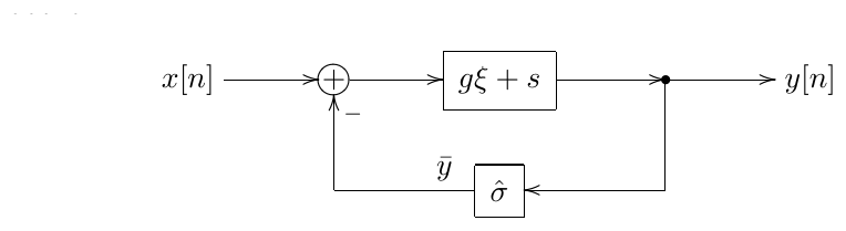
Figure 3.35: Digital 1-pole lowpass filter with a trapezoidal integrator in the instantaneous response form and a smoother unit in the delayless feedback path.
So, suppose we wish to compute a new output sample for the new input sample . At the time “arrives” at the filter’s input, the smoother still holds the old output value . Let’s freeze the discrete time at this point (which formally means we simply are not going to update the internal state of the element). At the same time we will let the continuous time run, formally starting at at the discrete time moment .
In this time-frozen setup we can choose arbitrary units for the continuous time . The smoother equation can be written as
That is, we don’t specify the details of the smoothing behavior, however the smoother output always changes in the direction from towards at some (not necessarily constant) speed.19 Particularly, we can simply define a constant speed smoother:
or we could use a 1-pole lowpass filter as a smoother:
The initial value of the smoother is apparently .
Now consider that
where is constant in respect to . First, assume . Further, suppose . Then and then the value of the expression will start decreasing until it turns to zero at some , at which point the smoothing process converges. On the other hand, if , then and the value of the expression will start increasing until it turns to zero at some , at which point the smoothing process converges. If then the smoothing is already in a stable equilibrium state.
So, in case the instantaneous feedback smoothing process always converges. Now assume . Further, suppose . Then and then the value of the expression will start further increasing (or stay constant if ). Thus, will grow indefinitely. Respectively, if , then will decrease indefinitely. This indefinite growth/decrease will occur within the frozen discrete time. Therefore we can say that grows infinitely in an instant. We can refer to this as to an instantaneously unstable zero-delay feedback loop.
The idea of the smoother introduced in Fig. 3.35 can be used as a general means for analysing zero-delay feedback structures for instantaneous instability. We will refer to this technique as instantaneous smoother.
1-pole lowpass as an instantaneous smoother
The analysis of the instantaneous stability can also be done using the analog filter stability analysis means. Let the smoother be an analog 1-pole lowpass filter with a unit cutoff (whose transfer function is )20 and notice that in that case the structure in Fig. 3.35 can be redrawn as in Fig. 3.36. This filter has two formal inputs and and one output .
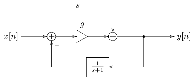
Figure 3.36: An instantaneous representation of a digital 1-pole lowpass filter with a trapezoidal integrator and an analog lowpass smoother.
We can now e.g. obtain a transfer function from the input to the output. Ignoring the input signal (assuming it to be zero), for a continuous-time complex exponential input signal arriving at the input, which we denote as , we have a respective continuous-time complex exponential signal at the output, which we denote as :
from where
that is
This transfer function has a pole at . Therefore, the structure is stable if and not stable otherwise.
The same transfer function analysis could have been done between the input and the output, in which case we would have obtained
The poles of this transfer function however, are exactly the same, so it doesn’t matter.21
Generalized zero-delay feedback loop
The zero-delay feedback instantaneous response structure in Fig. 3.29 can be considered as a particular case of a general one, drawn in Fig. 3.37, where the input signal has been incorporated into the term of the instantaneous response and the negative feedback has been incorporated into the factor . Indeed, Fig. 3.37 can be obtained from Fig. 3.29 via
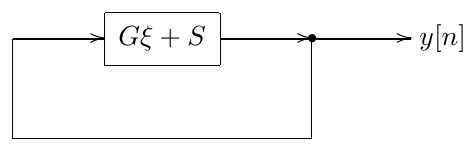
Figure 3.37: General zero-delay feedback structure in the instantaneous response form.
The zero-delay feedback equation solution written for Fig. 3.37 is obviously
From the previous discussion it should be clear that the structure becomes instantaneously unstable for , that is when the total instantaneous gain of the feedback loop is 1 or more.
The solution form (3.37) therefore provides a generic means to check an arbitrary zero-delay feedback loop for instantaneous instability. E.g. rewriting (3.28) (which we had written for Fig. 3.29) in the form (3.37) we obtain
where is the total instantaneous gain of the feedback loop (including the feedback inversion), and thus the structure is instantaneously unstable at (or, equivalently, ).
It might be tempting to simply say that the instantaneously unstable zero-delay feedback occurs whenever the denominator of the zero-delay feedback equation’s solution becomes zero or negative. However, this actually depends on how did we arrive at the solution expression. E.g. if we multiply both the numerator and the denominator of (3.28) by , the instantaneously unstable case will occur for zero or positive denominator values. Therefore, we need to make sure that our solution is written in the form (3.37) (where we need to verify that is the total instantaneous gain of the feedback loop) and only then can we say that zero or negative denominator values correspond to instantaneously unstable feedback.
Limits of bilinear transform
We have seen that for 1-poles the continuous- and discrete-time transient responses are
where the discrete-time pole is obtained from continuous-time pole via inverse bilinear transform (3.9).
In order to compare the transient responses we could compare the growth of over one sampling period :
The comparison of vs. is done in Fig. 3.38.
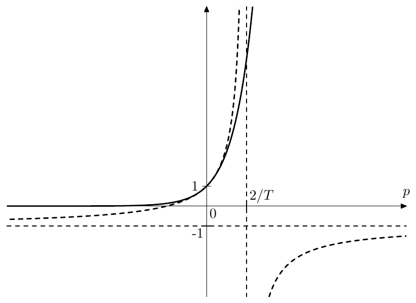
Figure 3.38: (solid) vs. (thick dashed) as functions of . The two thin dashed lines are asymptotes of .
One can notice that as the value of grows too quickly (compared to ), approaching infinity. This means that discrete-time transient response is growing infinitely fast at , or, respectively as . At the value of is getting completely different from , particulary the sign of begins to alternate between successive samples.
Now recall that in the 1-pole zero-delay feedback equation (3.28) we had . Thus, as the discrete-time transient response is becoming infinitely fast. Close to this point and further beyond it, trapezoidal integration doesn’t deliver a reasonable approximation to the continuous-time case anymore.
If we attempt to interpret the same in terms of bilinear transform, then we already know (Fig. 3.38) that the inverse bilinear transform (3.9) is becoming infinitely large at , that is the inverse bilinear transform formula has a pole at . This means that, if we are having a continuous-time system with a pole at (which in case of the 1-pole lowpass corresponds to ), then after the bilinear transform the system will have a pole at , and the transformation result doesn’t work really well.
Avoiding instantaneously unstable feedback
Alright, so we have found out that zero-delay feedback structures are instantaneously unstable when the total instantaneous gain of the feedback loop is greater than or equal to 1, but what can we do about it? Firstly, the problem typically doesn’t occur. Mostly, in (3.37) we have , e.g. in the 1-pole lowpass case we have for positive cutoff values. Even if is or can become positive, the situation occurs at really excessive parameter settings. Therefore one can consider, whether these extreme parameter settings are so necessary to support, and possibly simply clip the filter parameters in such a way that the instantaneous instability doesn’t occur.
Secondly, let’s notice that . Therefore another solution could be to increase the sampling rate, which reduces the sampling period and respectively the value of (from an alternative point of view, it shifts the inverse bilinear transform’s pole further away from the origin).
Unstable bilinear transform
There is yet another idea, which is not widely used, but we are going to discuss it anyway.22 So, the instantaneous instability is occurring at the moment when one of the analog filter’s poles hits the pole of the inverse bilinear transform (3.9), which is located at . On the other hand, recall that the bilinear transform is mapping the imaginary axis to the unit circle, thus kind-of preserving the frequency response. If the system is not stable, then the frequency response doesn’t make sense. Formally, the reason for this is that the inverse Laplace transform of transfer functions only converges for where are the poles of the transfer function, and respectively, if , it doesn’t converge on the imaginary axis (). However, instead of the imaginary axis , let’s choose some other axis and use it instead of the imaginary axis to compute the “frequency response”.
We also need to find a discrete-time counterpart for . Considering that defines the magnitude growth speed of the exponentials we could choose a -plane circle, on which the magnitude growth speed of is the same as for . Apparently, this circle is . So, we need to map to . Considering the bilinear transform equation (3.4), we divide by to make sure has a unit magnitude and shift the -plane result by :
We can refer to (3.38) as the unstable bilinear transform, where the word “unstable” refers not to the instability of the transform itself, but rather to the fact that it is designed to be applied to unstable filters.23 Notice that at the unstable bilinear transform turns into an ordinary bilinear transform. The inverse transform is obtained by
from where
and
Apparently the inverse unstable bilinear transform (3.39) has a pole at . In order to avoid hitting that pole by the poles of the filter’s transfer function (or maybe even generally avoid the real parts of the poles to go past that value) we could e.g. simply let
or we could position midways:
In order to construct an integrator defined by (3.38) we first need to obtain the expression for from (3.38):
That is
A discrete-time structure implementing (3.40) could be e.g. the one in Fig. 3.39. Yet another approach could be to convert the right-hand side of (3.40) to the analog domain by the inverse bilinear transform, construct an analog implementation of the resulting transfer function and apply the trapezoidal integrator replacement to convert back to the digital domain. It is questionable, whether this produces better (or even different) results than Fig. 3.39.
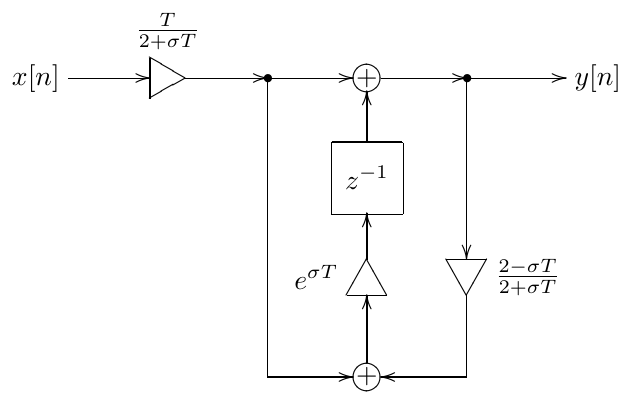
Figure 3.39: Transposed direct form II-style “unstable” trapezoidal integrator.
3.14 Other replacement techniques
The trapezoidal integrator replacement technique can be seen as a particular case of a more general set of replacement techniques. Suppose we have two filters, whose frequency response functions are and respectively. The filters do not need to have the same nature, particularly one can be an analog filter while the other can be a digital one. Suppose further, there is a frequency axis mapping function such that
Typically should map the entire domain of onto the entire domain of (however the exceptions are possible).
To make the subsequent discussion more intuitive, we will assume that is monotone, although this is absolutely not a must.24 In this case we could say that is obtained from by a frequency axis warping. Particularly, this is exactly what happens in the bilinear transform case (the mapping is then defined by the equation (3.6)). One cool thing about the frequency axis warping is that it preserves the relationship between the amplitude and phase.
Suppose that we have a structure built around filters of frequency response , and the rest of the structure doesn’t contain any memory elements (such as integrators or unit delays). Then the frequency response of this structure will be a function of :
where the specifics of the function will be defined by the details of the container structure. E.g. if the building-block filters are analog integrators, then . For the filter in Fig. 2.2 we then have
Indeed, substituting into we obtain
which is the already familiar to us frequency response of the analog lowpass filter.
Now, we can view the trapezoidal integrator replacement as a substitution of instead of , where is obtained from (3.6):
The frequency response of the resulting filter is obviously equal to , where is the frequency response of the trapezoidal integrators (used in place of analog ones). But since .
which means that the frequency response of the structure with trapezoidal integrators is obtained from the frequency response of the structure with analog integrators simply by warping the frequency axis. If the warping is not too strong, the frequency responses will be very close to each other. This is exactly what is happening in the trapezoidal integrator replacement and generally in the bilinear transform.
Differentiator-based filters
We could have used some other two filters, with their respective frequency responses and . E.g. we could consider continuous-time systems built around differentiators rather than integrators.25 The transfer function of a differentiator is apparently simply , so we could use (3.4) to build a discrete-time “trapezoidal differentiator”. Particularly, if we use the direct form II approach, it could look similarly to the integrator in Fig. 3.9. When embedding the cutoff control into a differentiator (in the form of a gain), it’s probably better to position it after the differentiator, to avoid the unnecessary “de-smoothing” of the control modulation by the differentiator. Replacing the analog differentiators in a structure by such digital trapezoidal differentiators we effectively perform a differentiator-based TPT.
E.g. if we replace the integrator in the highpass filter in Fig. 2.9 by a differentiator, we essentially perform a substitution, thus we should have obtained a (differentiator-based) lowpass filter. Remarkably, if we perform a differentiator-based TPT on such filter, the obtained digital structure is fully equivalent to the previously obtained integrator-based TPT 1-pole lowpass filter.
Allpass substitution
One particularly interesting case occurs when and define two different allpass frequency responses. That is and . In this case the mapping is always possible. Especially since the allpass responses (defined by rational transfer functions of analog and digital systems) always cover the entire phase range from to .26 In intuitive terms it means: for a filter built of identical allpass elements, we can always replace those allpass elements with an arbitrary other type of allpass elements (provided all other elements are memoryless, that is there are only gains and summators). We will refer to this process as allpass substitution. Whereas in the trapezoidal integrator replacement we have replaced analog integrators by digital trapezoidal integrators, in the allpass substitution we replace allpass filters of one type by allpass filters of another type.
We can even replace digital allpass filters with analog ones and vice versa. E.g., noticing that elements are allpass filters, we could replace them with analog allpass filters. One particularly interesting case arises out of the inverse bilinear transform (3.9). From (3.9) we obtain
The right-hand side of (3.41) obviously defines a stable 1-pole allpass filter, whose cutoff is . We could take a digital filter and replace all elements with an analog allpass filter structure implementing (3.41). By doing this we would have performed a topology-preserving inverse bilinear transform.
We could then apply the cutoff parametrization to these underlying analog allpass elements:
so that we obtain
The expression can be also rewritten as , where is the cutoff scaling factor:
Finally, we can apply the trapezoidal integrator replacement to the cutoff-scaled analog filter, converting it back to the digital domain. By doing so, we have applied the cutoff scaling in the digital domain! On the transfer function level this is equivalent to applying the bilinear transform to (3.42), resulting in
That is, we have obtained a discrete-time allpass substitution
which applies cutoff scaling in the digital domain.27 The allpass filter
should have been obtained, as described, by the trapezoidal integrator replacement in an analog implementation of (3.42), alternatively we could use a direct form implementation. Notice that this filter has a pole at . Since , the pole is always located inside the unit circle, and the filter is always stable.
Summary
We have considered three essentially different approaches to applying time-discretization to analog filter models: naive, TPT (by trapezoidal integrator replacement), and the classical bilinear transform (using direct forms). The TPT approach combines the best features of the naive implementation and the classical bilinear transform.
-
As with Laplace transform, sometimes there are no restrictions on the radius of the circle, sometimes there are. ↩
-
A more common term for (3.1) is the inverse z-transform, but we will prefer the z-integral term for the same reason as with Fourier and Laplace integrals. ↩
-
Formally the parameter of the Laplace integral (and z-integral) should have been multiplied by as well, but it doesn’t matter, since this parameter is chosen rather arbitrarily. ↩
-
Alternatively, we could, of course, scale the integrator’s output by , but this is less useful in practice, because the factor will be usually combined with the cutoff gain factor preceding the integrator. ↩
-
Based on the fact that the naive integration introduced above is identical to Euler backward-difference integration, there is an opinion that the naive approach (loosely defined as “take whatever values we have now at the integrator inputs and apply a single naive integration step to those”) is identical to the Euler method. This is not 100% so. The readers are encouraged to formally apply backward- and forward-difference Euler methods to to convince themselves that there are some differences. Particularly, the backward-difference method is implicit (requires solving an equation), while the forward-difference method produces the “future” value of the output. For more complicated systems the differences could be more drastic, although the author didn’t explicitly verify that. ↩
-
Under the assumption of causality, which holds if the system is built of unit delays. ↩
-
As in continuous-time case, we take for granted the fact that complex exponentials are eigenfunctions of discrete-time linear time-invariant systems. ↩
-
Another way to look at this is to notice that in order for to be a complex sinusoid we need to let . ↩
-
Many engineers seem to believe that the deviations in phase response are quite tolerable acoustically. The author’s personal preference is to be on the safe side and not take the risks which are difficult to estimate. At least some caution in this regard would be recommended. ↩
-
Difference systems can be defined as those, whose block diagrams consist of gains, summators and unit delays. More precisely those are causal difference systems. There are also difference systems with a lookahead into the future, but we don’t consider them in this book. ↩
-
A similar mapping obviously occurs for the negative frequencies. ↩
-
Note that thereby, should we become interested in the amplitude and phase responses of Fig. 3.12, we don’t have to derive the discrete-time transfer function of Fig. 3.12. Instead we can simply take the amplitude and phase responses of the analog 1-pole (which are simpler to compute) and apply the mapping (3.7). This is the reason that we almost exclusively deal with analog transfer functions in this book, we simply don’t need digital ones most of the time. ↩
-
Apparently, the picture in Fig. 3.13 will be the same at any other sampling rate, except that the frequency axis values will need to be relabelled proportionally to the sampling rate change. E.g. at 88.2kHz the labels would be 4, 8, 16, 22.05, 32 and 44.1kHz respectively. We could have labelled the axis in terms of normalized instead, but giving the absolute values is more illustrative. Particularly, the audible frequency range is easier to see. ↩
-
Notice that the choice of the signal point for the prediction is rather arbitrary. We could have chosen any other point within the delayless feedback loop. ↩
-
Apparently, naive filter design techniques also preserve the topology, but they do a rather poor job on the transfer functions. Classical bilinear transform approach does a good job on the transfer function, but doesn’t preserved the topology. The topology-preserving transform achieves both goals simultaneously. ↩
-
This is related to the fact that transfer functions can be defined only for linear time-invariant systems. Nonlinear cases are obviously not linear, thus some critical information can be lost, if the conversion is done solely based on the transfer functions. ↩
-
A higher-order transfer function is typically decomposed into a product of transfer functions of 1st- and 2nd-order rational functions (with real coefficients!). Then it can be implemented by a serial connection of the respective 1st- and 2nd-order direct form filters. ↩
-
Of course, such lowpass filter formally has a negative cutoff value. It is also unstable. However unstable circuits are very important as the linear basis for the analysis and implementation of e.g. nonlinear self-oscillating filters. Therefore we wish to be able to handle unstable circuits as well. ↩
-
We also assume that the smoothing speed is sufficiently large to ensure that the smoothing process will converge at all cases where it potentially can converge (this statement should become clearer as we discuss more details). ↩
-
Apparently, the variable used in the transfer function is a different than the one used in the instantaneous response expression for the integrator. The author apologizes for the slight confusion. ↩
-
This is a common rule: the poles of a system with multiple inputs and/or multiple outputs are always the same regardless of the particular input-output pair for which the transfer function is being considered (exceptions in singular cases, arising out of pole/zero cancellation are possible, though). ↩
-
This idea has occurred to the author during the writing of the first revision of this book. The author didn’t try it in practice yet, neither is he aware of other attempts.
Sufficient theoretical analysis is not possible here due to the fact that practical applications of instantaneously unstable (or any unstable, for that matter) filters occur typically for non-linear filters, and there are not many theoretical analysis means for the latter. Hopefully there are no mistakes in the theoretical transformations, but even if there are mistakes, at least the idea itself could maybe work. ↩
-
Apparently, the unstable bilinear transform defines the same relationship between and as the ordinary bilinear transform. Therefore prewarping can be done in the same way as for the ordinary bilinear transform. ↩
-
Strictly speaking, we don’t even care whether is single-valued. We could have instead required that for some and . ↩
-
The real-world analog electronic circuits are “built around” integrators rather than differentiators. However, formally one still can “invert” the causality direction in the equations and pretend that is defined by , and not vice versa. ↩
-
Actually, for , they cover this range exactly times, where is the order of the filter. ↩
-
Differently from the analog domain, the digital cutoff scaling doesn’t exactly shift the response along the frequency axis in a logarithmic scale, as some frequency axis warping is involved. The resulting frequency response change however is pretty well approximated as shiting in the lower frequency range. ↩