Chapter 1: Fourier theory

When we are talking about filters we say that filters modify the frequency content of the signal. E.g. a lowpass filter lets the low frequencies through, while suppressing the high frequencies, a highpass filter does vice versa etc. In this chapter we are going to develop a formal definition¹ of the concept of frequencies “contained” in a signal. We will later use this concept to analyse the behavior of the filters.

1.1 Complex sinusoids

In order to talk about the filter theory we need to introduce complex sinusoidal signals. Consider the complex identity:

$$e^{jt}=\cos t+j\sin t(t\in \mathbb{R})$$

(notice that, if $t$ is the time, then the point $e^{jt}$ is simply moving along a unit circle in the complex plane). Then

$$\cos t=\frac{e^{jt}+e^{-jt}}{2}$$

and

$$\sin t=\frac{e^{jt}-e^{-jt}}{2j}$$

Then a real sinusoidal signal $a\cos (\omega t+\phi )$ where $a$ is the real amplitude and $\phi$ is the initial phase can be represented as a sum of two complex conjugate sinusoidal signals:

$$a\cos (\omega t+\phi )=\frac{a}{2}\left(e^{j(\omega t+\phi )}+e^{-j(\omega t+\phi )}\right)=\left(\frac{a}{2}{e}^{j\phi }\right)e^{j\omega t}+\left(\frac{a}{2}{e}^{-j\phi }\right)e^{-j\omega t}$$

Notice that we have a sum of two complex conjugate sinusoids $e^{\pm j\omega t}$ with respective complex conjugate amplitudes $(a/2)e^{\pm j\phi }$. So, the complex amplitude simultaneously encodes both the amplitude information (in its absolute magnitude) and the phase information (in its argument). For the positive-frequency component $(a/2)e^{j\phi }\cdot e^{j\omega t}$, the complex “amplitude” $a/2$ is a half of the real amplitude and the complex “phase” $\phi$ is equal to the real phase.

1.2 Fourier series

Let $x(t)$ be a real periodic signal of a period $T$:

$$x(t)=x(t+T)$$

Let $\omega =2\pi /T$ be the fundamental frequency of that signal. Then $x(t)$ can be represented² as a sum of a finite or infinite number of sinusoidal signals of harmonically related frequencies $jn\omega$ plus the DC offset term³ $a_0/2$:

$$x(t)=\frac{a_0}{2}+\sum _{n=1}^{\infty }{a}_n\cos (jn\omega t+{\phi }_n)\text{\hspace{1em}(1.1)}$$

The representation (1.1) is referred to as real-form Fourier series. The respective sinusoidal terms are referred to as the harmonics or the harmonic partials of the signal.

The set of partials contained in a signal (including the DC term) is referred to as the signal’s spectrum. Respectively, a periodic signal can be specified by specifying its spectrum.

Using the complex sinusoid notation the same can be rewritten as

$$x(t)=\sum _{n=-\infty }^{\infty }{X}_n{e}^{jn\omega t}\text{\hspace{1em}(1.2)}$$

where each harmonic term $a_n\cos (jn\omega t+{\phi }_n)$ will be represented by a sum of $X_n{e}^{jn\omega t}$ and $X_{-n}{e}^{-jn\omega t}$, where $X_n$ and $X_{-n}$ are mutually conjugate: $X_n=X_{-n}^{\ast }$. The representation (1.2) is referred to as complex-form Fourier series and respectively we can talk of a complex spectrum. Note that we don’t have an explicit DC offset partial in this case, it is implicitly contained in the series as the term for $n=0$.

It can be easily shown that the real- and complex-form coefficients are related as

$$\begin{array}{rl}{X}_n& =\frac{a_n}{2}{e}^{j{\phi }_n}(n>0)\\ X_0& =\frac{a_0}{2}\end{array}$$

This means that intuitively we can use the absolute magnitude and the argument of $X_n$ (for positive-frequency terms) as the amplitudes and phases of the real Fourier series partials.

Complex-form Fourier series can also be used to represent complex (rather than real) periodic signals in exactly the same way, except that the equality $X_n=X_{-n}^{\ast }$ doesn’t hold anymore.

Thus, any real periodic signal can be represented as a sum of harmonically related real sinusoidal partials plus the DC offset. Alternatively, any periodic signal can be represented as a sum of harmonically related complex sinusoidal partials.

1.3 Fourier integral

While periodic signals are representable as a sum of a countable number of sinusoidal partials, a nonperiodic real signal can be represented⁴ as a sum of an uncountable number of sinusoidal partials:

$$x(t)={\int }_0^{\infty }a(\omega )\cos (\omega t+\phi (\omega ))\frac{d\omega }{2\pi }\text{\hspace{1em}(1.3)}$$

The representation (1.3) is referred to as Fourier integral.⁵ The DC offset term doesn’t explicitly appear in this case.

Even though the set of partials is uncountable this time, we still refer to it as a spectrum of the signal. Thus, while periodic signals had discrete spectra (consisting of a set of discrete partials at the harmonically related frequencies), nonperiodic signals have continuous spectra.

The complex-form version of Fourier integral⁶ is

$$x(t)={\int }_{-\infty }^{\infty }X(\omega )e^{j\omega t}\frac{d\omega }{2\pi }\text{\hspace{1em}(1.4)}$$

For real $x(t)$ we have a Hermitian $X(\omega )$: $X(\omega )=X^{\ast }(-\omega )$, for complex $x(t)$ there is no such restriction. The function $X(\omega )$ is referred to as Fourier transform of $x(t)$.⁷

It can be easily shown that the relationship between the parameters of the real and complex forms of Fourier transform is

$$X(\omega )=\frac{a(\omega )}{2}{e}^{j\phi (\omega )}(\omega >0)$$

This means that intuitively we can use the absolute magnitude and the argument of $X(\omega )$ (for positive frequencies) as the amplitudes and phases of the real Fourier integral partials.

Thus, any timelimited signal can be represented as a sum of an uncountable number of sinusoidal partials of infinitely small amplitudes.

1.4 Dirac delta function

The Dirac delta function $\delta (t)$ is intuitively defined as a very high and a very short symmetric impulse with a unit area (Fig. 1.1):

$$\begin{array}{rl}& \delta (t)=\{\begin{array}{ll}+\infty & \text{if }t=0\\ 0& \text{if }t\ne 0\end{array}\\ & \delta (-t)=\delta (t)\\ & {\int }_{-\infty }^{\infty }\delta (t)dt=1\end{array}$$

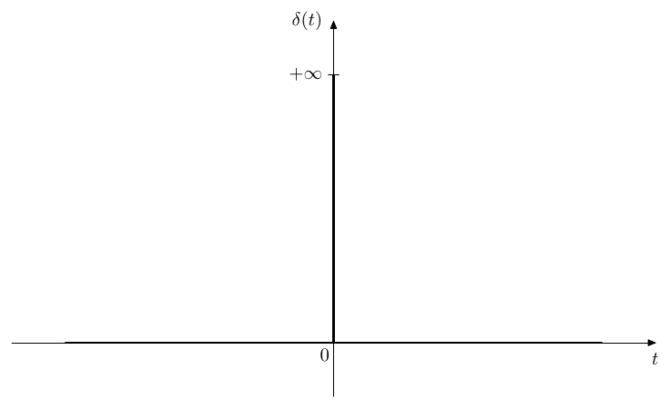
Figure 1.1: Dirac delta function.

Since the impulse is infinitely narrow and since it has a unit area,

$${\int }_{-\infty }^{\infty }f(\tau )\delta (\tau )d\tau =f(0)\forall f$$

from where it follows that a convolution of any function $f(t)$ with $\delta (t)$ doesn’t change $f(t)$:

$$(f\ast \delta )(t)={\int }_{-\infty }^{\infty }f(\tau )\delta (t-\tau )d\tau =f(t)$$

Dirac delta can be used to represent Fourier series by a Fourier integral. If we let

$$X(\omega )=\sum _{n=-\infty }^{\infty }2\pi \delta (\omega -n{\omega }_f)X_n$$

then

$$\sum _{n=-\infty }^{\infty }{X}_n{e}^{jn{\omega }_{f}t}={\int }_{-\infty }^{\infty }X(\omega )e^{j\omega t}\frac{d\omega }{2\pi }$$

Notice that thereby the spectrum $X(\omega )$ is discrete, even though being formally notated as a continuous function. From now on, we’ll not separately mention Fourier series, assuming that Fourier integral can represent any necessary signal.

Thus, most signals can be represented as a sum of (a possibly infinite number of) sinusoidal partials.

1.5 Laplace transform

Let $s=j\omega$. Then, a complex-form Fourier integral can be rewritten as

$$x(t)={\int }_{-j\infty }^{+j\infty }X(s)e^{st}\frac{ds}{2\pi j}$$

where the integration is done in the complex plane along the straight line from $-j\infty$ to $+j\infty$ (apparently $X(s)$ is a different function than $X(\omega )$).⁸ For timelimited signals the function $X(s)$ can be defined on the entire complex plane in such a way that the integration can be done along any line which is parallel to the imaginary axis:

$$x(t)={\int }_{\sigma -j\infty }^{\sigma +j\infty }X(s)e^{st}\frac{ds}{2\pi j}(\sigma \in \mathbb{R})\text{\hspace{1em}(1.5)}$$

In many other cases such $X(s)$ can be defined within some strip ${\sigma }_1<\mathrm{Re}s<{\sigma }_2$. Such function $X(s)$ is referred to as bilateral Laplace transform of $x(t)$, whereas the representation (1.5) can be referred to as Laplace integral.^{9 10}

Notice that the complex exponential $e^{st}$ is representable as

$$e^{st}=e^{\mathrm{Re}s\cdot t}{e}^{\mathrm{Im}s\cdot t}$$

Considering $e^{\mathrm{Re}s\cdot t}$ as the amplitude of the complex sinusoid $e^{\mathrm{Im}s\cdot t}$ we notice that $e^{st}$ is:

• an exponentially decaying complex sinusoid if $\mathrm{Re}s<0$,
• an exponentially growing complex sinusoid if $\mathrm{Re}s>0$,
• a complex sinusoid of constant amplitude if $\mathrm{Re}s=0$.

Thus, most signals can be represented as a sum of (a possibly infinite number of) complex exponential partials, where the amplitude growth or decay speed of these partials can be relatively arbitrarily chosen.

Summary

The most important conclusion of this chapter is: any signal occurring in practice can be represented as a sum of sinusoidal (real or complex) components. The frequencies of these sinusoids can be referred to as the “frequencies contained in the signal”. The full set of these sinusoids, including their amplitudes and phases, is refereed to as the spectrum of the signal.

For complex representation, the real amplitude and phase information is encoded in the absolute magnitude and the argument of the complex amplitudes of the positive-frequency partials (where the absolute magnitude of the complex amplitude is a half of the real amplitude). It is also possible to use complex exponentials instead of sinusoids.

1. More precisely we will develop a number of definitions. ↩

2. Formally speaking, there are some restrictions on $x(t)$. It would be sufficient to require that $x(t)$ is bounded and continuous, except for a finite number of discontinuous jumps per period. ↩

3. The reason the DC offset term is notated as $a_0/2$ and not as $a_0$ has to do with simplifying the math notation in other related formulas. ↩

4. As with Fourier series, there are some restrictions on $x(t)$. It is sufficient to require $x(t)$ to be absolutely integrable, bounded and continuous (except for a finite number of discontinuous jumps per any finite range of the argument value). The most critical requirement here is probably the absolute integrability, which is particularly fulfilled for the timelimited signals. ↩

5. The $1/2\pi$ factor is typically used to simplify the notation in the theoretical analysis involving the computation. Intuitively, the integration is done with respect to the ordinary, rather than circular frequency: $$x(t)={\int }_0^{\infty }a(f)\cos (2\pi ft+\phi (f))df$$ Some texts do not use the $1/2\pi$ factor in this position, in which case it appears in other places instead. ↩

6. A more common term for (1.4) is inverse Fourier transform. However the term inverse Fourier transform stresses the fact that $x(t)$ is obtained by computing the inverse of some transform, whereas in this book we are more interested in the fact that $x(t)$ is representable as a combination of sinusoidal signals. The term Fourier integral better reflects this aspect. It also suggests a similarity to the Fourier series representation. ↩

7. The notation $X(\omega )$ for Fourier transform shouldn’t be confused with the notation $X(s)$ for Laplace transform. Typically one can be told from the other by the semantics and the notation of the argument. Fourier transform has a real argument, most commonly denoted as $\omega$. Laplace transform has a complex argument, most commonly denoted as $s$. ↩

8. As already mentioned, the notation $X(\omega )$ for Fourier transform shouldn’t be confused with the notation $X(s)$ for Laplace transform. Typically one can be told from the other by the semantics and the notation of the argument. Fourier transform has a real argument, most commonly denoted as $\omega$. Laplace transform has a complex argument, most commonly denoted as $s$. ↩

9. A more common term for (1.5) is inverse Laplace transform. However the term inverse Laplace transform stresses the fact that $x(t)$ is obtained by computing the inverse of some transform, whereas is this book we are more interested in the fact that $x(t)$ is representable as a combination of exponential signals. The term Laplace integral better reflects this aspect. ↩

10. The representation of periodic signals by Laplace integral (using Dirac delta function) is problematic for $\sigma \ne 0$. Nevertheless, we can represent them by a Laplace integral if we restrict $\sigma$ to $\sigma =0$ (that is $\mathrm{Re}s=0$ for $X(s)$). ↩